Open again the first example of image pair in UVMAT_DEMO01_pair.(accessible on ​http://servforge.legi.grenoble-inp.fr/pub/soft-uvmat/).

Visual check

Particle Image Velocimetry (PIV) measures the displacement of features in a pair of images. Visual evidence of feature displacement between the two images is a prerequisite for the success of the computation. To observe this motion, write the file indices 1 and 2 in the boxes [i1] and [i2] respectively, in the frame [File Indices] on the left. Then push the red button [<-->] in the frame [Navigate], see figure. The image then alternatively switches from 1 to 2. The speed of motion can be adjusted with the slider [speed]. Press [STOP] to stop the motion.

<doc138|center>

Launching PIV

The PIV computation is accessed from uvmat by the upper bar command [Run/PIV], or from series by selecting the function civ_series. The name 'CIV' means Correlation Imaging Velocity to stress that the method relies on image correlation, which evaluates the displacement of image textures, not necessarily from particles. Note that an older GUI 'civ' is also available, but not used here.

A new GUI 'cic_input' now appears. In the menu [ListCompareMode], keep the default option 'PIV'. Keep also the default option Di=0|1 for the image pair (menu tag [!ListPairCiv1]). Keep also the default parameters in the frame CIV1 and press OK.

The PIV operation depends on many parameters, but the default values proposed by the GUI provide a good first approach in many cases. Press [RUN] to get the result. The button is then colored in grey until the computation is finished. The operation produces a file with format netcdf, extension .nc, in a subdirectory called 'CIV' by default. The file name ends with index string '_1-2' indicating that it results from images 1 and 2. The file name and its status is indicated in a new figure civ_status. Press the file name to open it with uvmat, or use the browser of uvmat.

<doc137|center>

Visualizing the velocity fields

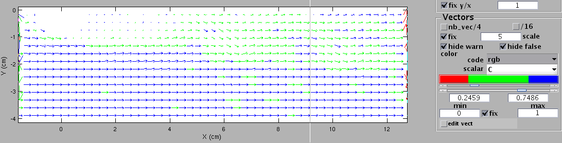
To read the velocity field, open it with the GUI 'uvmat'. Velocity vectors are displayed in the central window, while the histograms of each component are in the lower left windows, see Fig. [uvmat_fig]. The arrow length is automatically set by default. It can be adjusted by the edit box [VecScale] in the frame [Vectors'] on the right hand side.

The vector color indicates the quality of the image correlation maximum leading to each vector, blue is excellent, green average, red poor. The thresholds for such color display can be adjusted from 0 to 1 (perfect image correlation) in the frame [Vectors], using the boxes [!ColCode1] and [!ColCode2], or equivalently by the corresponding sliders [Slider1] and [Slider2] .

Vector color can also represent another quantity, as chosen in the menu [ColorScalar] in the frame [Vectors]. For instance the vector length norm_vec can be used. Then a color continuous 64 color code is appropriate, as set in the menu [ColorCode]. The color codes values between the valuies set by [MinVec] and [MaxVec].

The position (x,y) and velocity components (U,V) can be displayed in the upper right text display window by moving the mouse over it.

Derived fields

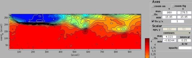
Other field representations are available, selected in the menu [Fields] at the top of the GUI. For instance the option 'u' provides a (false) color map of the x wise velocity component. A contour plot can be obtained instead of a color map by selecting the option 'contour' in the menu [ListContour?] in the frame [Scalar] . Then select the contour interval, for instance 0.5. The result is shown in the following figure. <doc145|center>

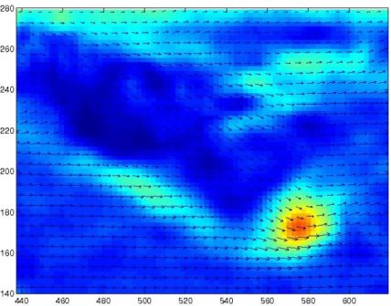
To get the vorticity field, 'vort' , and other spatial derivatives, you need to come back to the GUI CIV, select the check boxes [FIX1] and [PATCH1] , and press [RUN]. This will produce an interpolated velocity field and their spatial derivatives in the same netcdf file. After this operation vorticity can be visualized in the GUI uvmat, selecting the option [vort] in the popup menu [Fields]. The color code can be adjusted by the edit box [MinA] (saturated blue color below this value) and [MaxA] (saturated red color beyond this value).

Superposing image and vectors

It can be useful to visually superpose the images to the velocity field. This is done by selecting the option 'image' in the popup menu [Fields_1], located just under the popup menu [Fields] in the upper frame [Input]. To remove the image, select the blank option in [Fields_1] .

Similarly, the velocity vectors can be superposed to the vorticity field, selecting [vort] in [Fields_1] instead of [image .

Profiles

The velocity profile along a line can be obtained by creating a line with the upper menu bar [Projection object/line]. Then press the left hand side mouse button and draw the line, keeping the button pressed. Release the button to stop the drawing. The transverse and longitudinal velocity components along this line are then plotted in a new figure view_field.

Histograms

The global histograms of the displayed quantities (vector components or image brightness) are available in the lower left windows. Histograms limited to a sub-region can be extracted by the menu bar tool [Projection object], selecting either [rectangle], [ellipse] or [polygon] to define the sub-region. Then draw the contour with the mouse, like for line profiles.