
| Version 94 (modified by , 12 years ago) (diff) |
|---|
--- Help for Uvmat ---
TracNav
- 1 - Generalities
- 2 - Overview of the GUI uvmat
- 3 - Input files and navigation with uvmat
- 4 - Scalar and vector display
- 5 - Field structures
- 6 - Projection objects
- 7 - Netcdf files and the GUI get_field
- 8 - Geometric calibration
- 9 - Masks and grids
- 10 - Processing field series
- 11 - PIV: Particle Imaging Velocimetry
- 12 - Tridimensional features
- 13 - Editing xml files with the GUI editxml
- 14 - Appendix: overview of the package functions
1 - Generalities
1.1 Aim
The package uvmat can be used to visualise, scan and analyse a wide variety of input data: all image and movie formats recognised by Matlab (see section 3.1), NetCDF binary files(see section 7). It is however particularly designed for laboratory data obtained from imaging systems: it includes a Particle Image Velocimetry software, as well as tools for geometric calibration, masks, grid generation and image pre-processing (e.g. background removal), and editing documentation files in the format xml. Stereoscopic PIV, PIV-LIF and 3D PIV in a volume (still under development) are handled.
This package can be used without knowledge of the Matlab language, but it is designed to be complemented by user defined Matlab functions, providing flexibility for further data analysis. It provides convenient tools to develop a set of processing functions with a standardised system for input-output.
Installation is described in http://servforge.legi.grenoble-inp.fr/projects/soft-uvmat/wiki#UVMAT.
1.2 The package
The master piece is a Matlab GUI, made of a Matlab figure uvmat.fig and an associated set of sub-functions in the file uvmat.m. The menu bar at the top of the GUI, push buttons and editing box in uvmat.fig activate the Matlab sub-functions (callback functions) in uvmat.m. The package also contains the following set of GUI.
- browse_data.fig: scans the data directory of a project
- editxml.fig: displays and edits xml files according to an xml schema. xml reading and editing is performed by the toolbox xmltree, integrated in the package uvmat as a subdirectory /@xmltree.
- geometry_calib.fig: determines geometric calibration parameters for relating image to physical coordinates. The toolbox http://www.vision.caltech.edu/bouguetj/calib_doc/ is used, integrated in the package uvmat as a subdirectory /toolbox_calib.
- get_field.fig: selects coordinates and field in a general NetCDF file.
- series.fig: applies various processing functions to series of fields. A set of functions is integrated in the package as a subdirectory /series, but new functions can be introduced by the user.
- set_object.fig: creates and edits geometric objects used to project data: points, lines, planes...
- view_field.fig: is a GUI complementing uvmat for plotting projected data.
Functions in the package are used to generate file names, to read files and plot data, and to perform various ancillary tasks. The full set of functions is listed in overview of the package.
1.3 Documentation and help
The present on-line document is the reference document for the version currently available on the svn server. Features not yet implemented or tested (in particular 3D features) are marked by . The document is accessible within Matlab by help buttons in the GUIs.
A short comment about each GUI element, called uicontrol (push buttons, edit boxes, menus..), as well as the tag name of this uicontrol, is provided as a tool tip window by moving the mouse over it. In the present help document, the tag of a GUI element is quoted as [ tag], a file name in the package is enhanced as fct name.m, and commands on the Matlab workspace as '>> command’. The tag name can be also obtained by pressing the right hand mouse button on the element.
Information is also provided as comments in each function. Type '>>help fct_name' to get it, or open it with an editor.
Finally a on-line tutorial is provided with test images and data files.
1.4 Copyright and licence
Copyright Joel Sommeria, 2008, LEGI / CNRS-UJF-INPG, joel.sommeria(at)legi.grenoble-inp.fr.
The package UVMAT is free software; it can be redistributed and/or modified it under the terms of the GNU General Public License as published by the Free Software Foundation; either version 2 of the License, or (at your option) any later version.
UVMAT is distributed in the hope that it will be useful, but WITHOUT ANY WARRANTY; without even the implied warranty of MERCHANTABILITY or FITNESS FOR A PARTICULAR PURPOSE. See theGNU General Public License (file {COPYING.txt}) for more details.
2 - Overview of the GUI uvmat.fig
2.1 Opening the GUI
Type '>>uvmat' in the Matlab prompt to display the GUI. If the function is unknown by Matlab, add the appropriate path to the folder UVMAT where the toolbox has been installed (see the Matlab command '>>help path'). When the GUI is opening, the date of last modfication is displayed in the central window. During opening, the program checks the Matlab path to all the functions of the package (using the function check_functions.m). If a function is missing, or if it is overridden by a function with the same name at another path location, a message is displayed in the central window at the opening of the GUI uvmat.fig. Finally, if the svn server is accessible by line-command, the latest version number of the uvmat package is indicated.
The GUI contains an upper menu bar, a central graphic display window, a lower left window for histogram, a top right text display window, columns of edit boxes and command buttons on both side.
Each of the graphic elements (uicontrols) is described by a tag name, which can be displayed by moving the mouse over it: a tool tip window appears with the tag name followed by a short help description. The element tag and content can be also displayed in a zoom window, and possibly edited there, by a right hand mouse selection on the element. As a rule, tag names for checkboxes begins by 'Check', while tags of elements with numerical content begins by num_.
The red pushbuttons command the main actions. The color of pushbuttons or other elements turns to yellow while their callback function is active.
")
2.2 The upper menu bar
The menu bar at the top of the GUI contains the following buttons:
- [Open]: gives access to the browser for the main input field.
- [browse...]: open a general file browser browser_uvmat. In the displayed list, a file can be selected for opening (by a single mouse click),or directories are marqued by '+/'. Select the first line '+/..' to move up in the directory tree, and the arrow <-- to move backward. The dates of file creation can be displayed by pressing the button [dates]. file ordering by name or date can be chosen by the popumenu above. A path can be directly entered by copy-paste in the upper edit window of the browser.
- Previously opened files are memorised in the menu where they can be selected again.
- [Open campaign] : scan the data organised as a project/campaign, see section 3.7.
- Previously opened campaigns are memorised in the menu where they can be selected again.
- [Export] : used to export the currently displayed data, either as array structure in the Matlab workspace, either as a figure or a movie (for a succession of views), or plotted on an existing figure (axes) for comparison with previous data.
- [Projection object] : used to create projection objects (points, lines, patches, gridded planes) for data analysis and interpolation, see section 6.
- [Tools]:
- [Geometric calibration] for geometric calibration of images
- [LIF calibration]: calibration of images for Laser Induced Fluorescence
- [Make mask]: for creating mask images (for PIV)
- [Make grid]:: for making measurement grids for PIV
- [ruler]: displays a ruler to measure lengths and angles of any line.
- [Run] :
- [field series]: gives access to the GUI 'series.fig' for processing field series.
- PIV : gives access to the PIV program under Matlab (using the GUI series.fig).
- [CivX(Fortran)]: gives access to the GUI 'civ.fig' for Particle Imaging Velocimetry (CivX version in Fortran).
- [Help] : displays this help file using the Matlab browser.
2.3 Displaying the input file name
After selection by the browser, the path and file names are determined. The path is split into the two first edit boxes [RootPath] and [SubDir], while the file name is split into a root name [RootFile], file index string [FileIndex], and file extension [FileExt]. The input file name can be directly entered and modified in these edit boxes, without the browser.
Once a root name has been introduced, navigation among the file indices is provided by the red push buttons [runplus] ( [+>]) and [runmin] ([<-]). The central push button [run0] ([!0]) refreshes the current plot. See section 3.4 for more details.
When available, the time of each frame or field is displayed in the edit box [TimeValue], at the very right. In the case of image pairs, the time interval Dt is displayed between the edit boxes [i1], [j1] and [i2], [j2]. This timing information can be read directly in the input file, in the case of movies or Netcdf files, or can be defined in a xml documentation file, see section 3.5 (in case of conflict, the latter prevails).
Note: the five last input file names, as well as other pieces of personal information, are stored for convenience in a file (uvmat_perso.mat) automatically created in the user preference directory of Matlab (indicated by the Matlab command '>>prefdir'. Browsers then read default input in this file. A corruption of this file uvmat_perso.mat may lead to problems for opening uvmat, type '>>reinit' on the Matlab prompt to delete it and reinitialise the configuration of uvmat.
2.4 General tools
- Mouse motion: the local coordinates and field values are obtained by moving the mouse over a plotting axes. They are displayed in the text box [text_display] on the upper right.
- Zoom: is activated by selecting the check box [CheckZoom] on the upper right. Zoom in by pressing the left mouse button on the graph. Zoom out by pressing the right mouse button. Alternatively, a zoomed region can be displayed as a separate figure by selecting [CheckZoomFig] and drawing a rectangle with the mouse. The zoomed region can be translated through the initial field by pressing the directional arrows of the keyboard.
- Graph limits: they automatically adjust to the field when the check box [CheckFixLimits] is not selected (default). Otherwise they remain fixed, and can be adjusted by the check boxes [num_MinX], [num_MaxX], [num_MinY], [num_MaxY].
- Coordinate aspect ratio: when [CheckFixAspectRatio] is selected (the default option for images), the scale ratio for the x and y coordinates is fixed to 1 by default (it can be manually adjusted by the edit box [num_AspectRatio]. When [CheckFixAspectRatio] is not selected the graph scales along x and y automatically adjust to the figure size.
- Extracting graphs: The graph displayed in the central window can be copied to a separate figure by pressing the menu bar command [Export/extract figure]. This allows plot editing, exporting in image format and printing, using standard Matlab graphic tools. Plots can be also exported on an existing figure for data comparison, using the option [Export/export on axis]. A movie can be produced using the command [Export/make movie avi].
- Extracting data as Matlab arrays. Information stored in the GUI uvmat (as UserData in the figure) can be extracted in the Matlab work space by the menu bar command [Export/field in workspace] (or by pressing the right mouse button on the GUI). Type '>>Data_uvmat.Field' to get the current input field as a Matlab structure. An image or scalar matrix is for instance obtained as Data_uvmat.Field.A.

3 - Input files and navigation with uvmat
3.1 Input data formats
uvmat can read any image format recognised by the Matlab image reading function imread.m. Images can be in true color or B&W, with 8 bit or 16 bit grey levels. Image files containing multiple frames are handled. Movie files can be also opened, using the Matlab function VideoReader.m, or mmreader.m for older versions of Matlab.
Uvmat can also read various kinds of data in the binary format Netcdf, as described in section 7. Velocity fields obtained by PIV and results of data processing are stored in this format. Derived quantities (vorticity, divergence...) can be directly obtained. The input file type is recognized by the function get_file_type.m of uvmat and the file is opened by the function read_field.m according to this file type. It is possible to include new input file types by a modification of these two functions.
The PIV software provided in uvmat can deal with any image or movie format recognised by Matlab, while the older fortran version CIVx requires B&W images in the format png (portable network graphics). It is a binary format for images with lossless (reversible) compression, recommended by w3c (http://www.w3.org/Graphics/PNG). It is an open source patent-free replacement of GIF and can also replace many common uses of TIFF. It can be read directly by all standard programs of image visualisation and processing. Compressing a raw binary image to its png form typically saves disk storage by a factor of 3.
For 3D PIV, 'volume' images, with file extension .vol are used. These are images in the png format, where the npz slices are concatenated along the y direction, forming a composite image of dimension (npy x npz, npx) from the images (npy x npx).
3.2 Selecting fields from CIV
To update... The package uvmat recognizes the NetCDF fields obtained from the CIVx software. This includes the velocity fields and their spatial derivatives, as well as information about the CIV processing (image correlation values and flags). The vorticity, divergence, or strain are read in the same NetCDF files, but are available only after a PATCH operation has been run in the CIVx software, see section 11.
<doc71|center>
When a CIV field is recognised, the popup menu [Fields] is set by default to 'velocity' while a menu [VelType] (with items 'civ1', 'filter1',..) appears at the upper right of the GUI.
The choice can be imposed by selecting a check box, or can be left automatic. The second iteration (civ2, filter2), presumed to be of higher quality, is prefered by default. The filter fields are interpolated on a regular grid, with or without smoothing respectively. It allows to fill holes and get spatial derivatives. If a scalar depending on spatial derivatives, like vort, is selected, the field option switches automatically from civ to filter.
The choice of fields, velocity, vorticity, divergence... is done by the popup menu [Fields]. The option 'image' gives access to an image file corresponding to the velocity field. The option 'get_field...' allows the user to display all the variables of the netcdf file in the GUI get_field.fig. This is the only available option when the input file is not from CIV.
3.3 File naming and indexing
Different kinds of file or image frame indexing are defined:
-Simple series: files in a series can be labeled by a single integer index i, with name obtained by concatenation of the full root RootPath/RootFile), an index string suffix, and the file extension FileExt (example Exp01/aa_45.png). A frame series can be alternatively read from a single movie file. Then the index i stands for the frame index within the file.
-Double index series: they are labeled by two integer indices i and j. This double index labeling is commonly used for bursts of images (index j or equivalently a letter appendix 'a', 'b') separated by longer time intervals (index i). It can be also used for successive volume scanning by a laser sheet, with index j representing the position in the volume and i the time. For a set of indexed movies (or multimage files), the index i labels the files while the index j labels the frames within a file.
-Pair indexing: new file series can result from the processing of primary series. For a sequential processing limited to a single file, the output index naturally reproduces the input index. Other processing functions involve pairs of input files, for instance Particle Imaging Velocity from image pairs. In a simple series, the result from the two primary fields *_i1 and *_i2 is then labeled as *_i1-i2 with the file extension indicating the output format. More generally, the result from any processing involving a range of primary indices from i1 to i2 is labeled as _i1-i2. If i1=i2 or j1=j2, the two indices are merged in a single label i, or j respectively.
-Nomenclature types: The nomenclature type is defined as the character string representing the index (or indices) for the first file in the series, for instance '_1' for a single indexing and '_1-2' for a pair indexing, '_1_1' for a double index series. The second index j can be also represented as a letter suffix, for instance '01a'. For a field series in a single file, like a movie, the nomenclature type is defined as '*'. The functions fullfile_uvmat.m generates a file name from a root name, four numerical indices i1,i2,j1,j2 and the nomenclature type. The reverse operation, splitting a name into a root and indices while detecting the nomenclature type, is performed by the function fileparts_uvmat.m. The function find_file_series.m is also needed to scan the whole file series, leading to a possible adjustement of the nomenclature type (for instance distinguishing '_001' from '_1' when the file with index 1000 has been opened). Once the nomenclature type has been detected by the browser of uvmat.fig, it is displayed in the edit box [NomType] and used to generate all the file names when the series is scanned.
3.4 Navigation among field indices
The field indices can be incremented or decremented by the push buttons [runplus] ( +) and [runmin] (-) respectively. This scanning is performed over the first index (i) or the second one (j), depending on the selection of the check boxes [scan_i] or [scan_j] respectively. The step for increment is set by the edit box [increment_scan]. If this box is blank (or does not contain a number) the next available file is opened.
<doc65|center>
The current indices are displayed in the four edit boxes [i1], [i2], [j1], [j2]. The two first indices i1 and j1 are used for image series, while the second line i2, j2 is used to label the image pairs used for PIV data. The file indices can be directly set in these edit boxes, or equivalently in the edit box [FileIndex] at the top of the GUI.
For navigation with index pairs, the reference index, defined as the integer part of the mean value ((j1+j2)/2), is incremented. If the check box [fix_pair] is selected, the difference j1-j2 is then fixed while the reference index i or j is incremented. Else the pair with appropriate reference index is searched. In the case of multiple choices, the most largest index interval is chosen. This allows us to scan successive fields obtained with different image pairs (to deal with time evolving velocity fields).
The maximum value detected for each index is indicated by the boxes [last_i] and [last_j] respectively.
-slices: Images may be obtained with laser scanning in a multilayer mode, introducing a periodicity for the index i. This can be accounted by pressing the pushbutton [slices] and introducing the period in the edit box [num_NbSlice] which then appears. The index i modulo nb_slice then appears in the edit box [z_index].
-Movie scan: Fields can be continuously scanned as a movie by pressing the pushbuttons [Movie] ( [++>]) or [MovieBackward] . The movie speed can be adjusted by the slider [speed]. Press [STOP] to stop the movie.
-Keyboard short cuts: the activation of the push buttons [runplus] and [runmin] can be performed by typing the key board letters 'p' and 'm' respectively, after the uvmat figure has been selected by the mouse. Similarly the command of the push button [run0] can be performed by typing the 'return carriage' key.
3.5 Image documentation files (.xml)
Image series in uvmat are documented by a file providing image timing, geometric calibration, camera type and illumination. This file is in the format xml, a hierarchically organised text file. The content is labelled by tags, represented by brackets <.>, whose names and organisation are specified by a schema file (.xsd). A general introduction to the xml language and schemas is provided for instance in http://www.w3schools.com/xml. The schema used for image documentation is ImaDoc.xsd, available in the uvmat package in a sub-directory /Schemas. Simple templates of xml files are also provided there.
When a new file series is opened in uvmat, the xml documentation file is automatically sought in the folder containing the data series folder: the documentation of the file series RootPath/SubDir/RootFile_1,... is in the file RootPath/RootFile.xml. As a second choice (corresponding to an earlier convention), the xml file will be sought inside the data series folder, as RootPath/SubDir/RootFile.xml (if this file does not exist, a text file with the same root name but extension .civ is sought as an obsolete option). The detection of the image documentation file is indicated by the visibility of the pushbutton [view_xml] on the upper right of the GUI uvmat.fig. Press this button to see the content through an xml editor editxml.fig (described in section 10). The xml file can be also opened directly by the uvmat browser, or by any text editor. In uvmat, it is read by the function imadoc2struct.m.
The xml file <ImaDoc> can contain the following sections, as prescribed by the schema file ImaDoc.xsd.:
- <Heading> contains elements <Campaign>, <Experiment>, <DataSeries>, which recall the position of the file in the tree structure of data files. This allows the user to check that the document file has not been displaced.
- <Camera> contains information on the camera settings, as well as the timing of all the images in a subsection <BurstTiming>.
- <TranslationMotor> and <Oscillator> contains information on the mechanical devices used to produce the laser sheet and scan volumes.
- <GeometryCalib> contains the parameters of the geometric calibration relating the pixel position to the real space coordinates (see section 8]). In the case of volume scanning, it also describes the set of laser plane positions and angles.
- <Illumination> describes the illumination system used, including the position of the laser source.
- <Tracor> describes the properties of the flow tracor (particle, dye...)
3.6 Ancillary input files
- Mask: Masks are used to avoid PIV computations in specified areas. The file is a B&W 8 bit png image, with the same size as the image it has to mask. The grayscale code used is :
- Intensity < 20: ('black mask') the vector in this place will be set to zero
- 20 < Intensity < 200:('gray mask') the vector in this place will be absent
- Intensity>200 the vector will be computed The mask corresponding to an image or velocity field can be displayed in uvmat.fig by selecting the check box [view_mask]([CheckMask?]) on the upper left. Images with appropriate name can be automatically recognised by uvmat.fig and civ functions, see section 9.1. Otherwise file selection by a browser is proposed when [view_mask] is selected.
- Grid: List of numbers (in ascii text) specifying the set of points where the PIV processing is performed. It specifies the number of points n and a corresponding list of x and y coordinates expressed in image pixels, as follows
n X1 Y1 X2 Y2 ...... Xn Yn
The coordinates correspond to the center of the correlation box on the first image of the pair (the actual vector position will be shifted by half the displacement found between the two images). A tool to create grids is described in section 9.2.
- .fig Matlab figures represent plots but also Graphic User Interfaces (GUI). In that case Matlab functions (callbacks) are attached to the graphic objects in the figure and can be activated by the mouse. Matlab figures can be directly opened by the browser of uvmat.fig.
- '.civ' (obsolete) ascii text file containing the list of image times and the scaling in pixels/cm. This is an obsolete version of the xml image documentation file. It is stored in the same directory as the corresponding series of images, with name root .civ. It is automatically sought by uvmat.fig and series.fig, in the absence of an xml file <ImaDoc>. (it is read by the function read_imatext.m). The following example is from an experience with 19 bursts of 4 images, named aa001a,aa001b,aa001c,aa001d,aa002a,aa002b,...,aa019c,aa019d, with an extension .png. The corresponding .civ file is named aa.civ. Comments (not included in the file) are indicated with %...
19                              % number of bursts
1024 1024                       % image size npx npy
4                               % number of images per burst
2                               % not used
0.016667                        % time of exposure (in seconds)
5.860000 5.860000               % scaling pixel/cm x and y directions
5.860000 5.860000               % same
0                               % not used
1 0.000000 30 60 30 1           % for each line: burst number; time elapsed in second from the beginning; number of frames
2 25.001003 30 60 30 1          % between image a and image b; number of frames between image b and image c; number of frames
 .........................      % between image c and image d; image acquisition duration in frames
18 424.999847 30 60 30 1
19 450.000824 30 60 30 1
- .cmx ascii text files containing the parameters sent by the GUI civ.fig to the CIV fortran programmes. Each velocity field named *.nc results from a parameter file *.cmx. It can be opened by the browser of uvmat.fig. In a later version of civx, the .cmx file is replaced by a .xml ’CivDoc’ file.
- .log ascii text files, containing information about processing in batch mode. Each velocity field named *.nc is associated with a file *.log. A file *_patch.log is similarly produced by the ’patch’ program. These files can be opened by the browser of uvmat.fig.
3.7 Data organisation in a project
The package is designed to foster a good data organisation. The raw data from a project should be organised as:
Project/Campaign/Experiment/DataSeries/data files.
- Project contains all information on a project.
- Campaign corresponds to a series of experiments obtained by varying a given set of physical parameters. A set of parameter names (with units) is expected to be associated to a campaign. A project may involve several campaigns corresponding to different configurations, hence different relevant parameters. For a single configuration, 'Campaign' can be at the top of the data tree, without an additional 'Project' level. The uvmat package does not manage levels above 'Campaign'.
- Experiment is a directory containing all the data for a particular experiment, defined by a choice of values for the physical parameters.
- DataSeries contains an image series or movie from a camera, or more generally a data series from a device. Its name must correspond to the device and remain the same for all the experiments using this device. The results from data processing, as provided by 'civ' or 'series', are stored at the same level in a DataSeries directory, named from the source one with a extension specific to the processing program, for instance '.civ' for the PIV data.
Mirror data trees can be created to process a source data set in 'read only' mode, to preserve the safety of the data source, and to allow several users to work in parallel without interference.
The data organisation can be controlled and managed by the GUI browse_data.fig. This is called by the menu bar option [Open/browse campaign] in uvmat: with this browser select the path of the folder considered as 'Campaign' (instead of the data file itself). Then the GUI browse_data.fig appears with a list of 'Experiments' and a list of 'DataSeries'. Select your choice to open the corresponding file series in uvmat.fig. The selected campaign path is then recorded for future opening under [Open/browse campaign] in the menu bar of uvmat.fig.
Instead of directly opening a file series with browse_data.fig, you can create a 'mirror data tree' by pressing 'create_mirror', then selecting the path chosen for the new mirror folder 'Campaign'. Inside this mirror folder, a set of folders is then created for each experiment. Furthermore, an xml file 'mirror.xml' is created to recall the source directory (under the label <SourceDir>). Inside each mirror folder 'Experiment', the source is reproduced as symbolic links. Data processing in the mirror campaign then produces 'real' DataSeries folders.
Once created, this mirror campaign folder can be opened instead of the source. It can be regularly updated from the source folder by pressing the button 'update_mirror' in browse_data.fig.
4 - Scalar and vector display
The uvmat interface primarily reads and visualises two-dimensional fields, which can be images or scalars, or vector fields.
4.1 Images and scalars:
Images are matrices of integers, visualised by the Matlab function imagesc.m. The number of pixels in x and y is indicated in the boxes [num_Npx] and [num_Npy] respectively. Note that while the x coordinate of the image ranges from 1/2 to npx-1/2, the pixel index in y ranges from the maximum ordinate npy-1/2 to the smallest one 1/2.
True color images are described by a matrix A(npy,npx,3) of integers between 0 and 255, the last index labeling the color component red, green or blue. They are displayed directly as color images.

The greyscale images are described by a matrix A(npy,npx) of positive integers. The luminosity range depends on the camera dynamics (0 to 255 for 8 bit images, 0 to 65535 for 16 bit images). Luminosity represented with grey levels, according to the colorbar displayed on the right. The luminosity and contrast can be adjusted using the edit boxes [num_MinA] and [num_MaxA] : the luminosity level set by [num_MinA] (and levels below) is represented as black, and the luminosity level set by [num_MaxA] (or levels above) as white. When the check box [CheckFixScalar] is not selected, these bounds are set automatically to the image minimum and maximum respectively. Then the image may appear dark if a single point is very bright, in that case a lower value must be set by [num_MaxA]. Greyscale images can be displayed with false colors, from blue to red, by unselecting the check box [CheckBW].
Note that greyscale images with low resolution are linearly interpolated on a finer mesh for nicer display. This interpolation can be also done as image processing by defining a grid on a projection object 'plane', see section 6.
Two images can be visually compared by switching back and forth between them as a short movie. This is quite useful to get a visual feeling of the image correlation for PIV. This effect is obtained by introducing two image indices in the edit boxes j1 and j2 (or i1 and i2), and selecting the button [movie_pair] ('[<-->]') to switch between these two indices. The speed of the movie can be adjusted by the slider [speed]. Press [movie_pair] again, or [STOP], to stop the motion.
Scalar fields are represented like greyscale images, by default with a false color map ranging from blue (minimum values) to red (maximum), or as gray scale images by selecting the check box [CheckBW]. Other color maps can be used by extracting the figure with the menu bar button [Export/extract figure], then using the standard Matlab button [Edit/Colormap] in the figure menu bar.
Scalar are represented by matrices with real ('double') values, unlike images which are integers. They can be alternatively defined with unstructured grid (see section 5.1): they are then linearly interpolated on a regular grid before visualisation (a fairly slow process).
4.2 Contour plots
Scalars (or image intensity) can be also represented with contour plots, by switching the popup menu [Contours] from the setting 'image' to the setting 'contours'. Contours for positive scalar values are in sold line while contours for negative values are dashed. The interval between contours can be set by the edit box [num_IncrA]. The interval is automatically determined if the box content is blank.
By default, the contours are further marked by jumps of color levels. This can be set to grey levels by selecting the check box [CheckBW]. To suppress these images, set [Opacity] to 0. '
4.3 Vectors
The vector fields are represented by arrows. The length of the arrows is automatically set by default, or can be adjusted by the edit box [num_VecScale] when the check box[CheckFixVectors] is selected. For clarity of visualisation, the number of displayed vectors can be divided by 2 or 4 in each direction by selecting the check box [CheckDecimate4], or [CheckDecimate16] respectively.
Each vector has a color, ranging from blue to red, which can represent an associated scalar value. In addition, black and magenta colors represent warning and error flags respectively. This color system is primarily designed for PIV data but can be used in other contexts as well.

-Warning flags: they indicate a vector resulting from a dubious image correlation process, but not removed from the data set. They are displayed in black by default. This feature can be desactivated by selecting the check box [CheckHideWarning].
-Error flags: they mark vectors considered as false. These vectors are kept in the data set so that their elimination can be reversed, but they must not be taken into account for data processing. These false vectors are displayed in magenta. They can be also removed from the plot by selecting the check box [CheckHideFalse].
-Associated scalar: for PIV velocity fields, the color represents by default the image correlation C, ranging from 0 to 1. The red values correspond to poor correlations, green to fair values, and blue to good ones. The value range covered by each of the three colors is set by the pair of sliders [Slider1] and [Slider2], or equivalently by the edit boxes [num_ColCode1] and [num_ColCode2]. Other color representations can be specified. [ColorScalar] sets the scalar used for color representation, for instance the vector norm 'norm_vec' or vorticity 'vort' (the list of available scalars is set by the function {calc_scal.m}).
-[ColorCode] sets the kind of color representation:
- 'rgb': color ranging from red, for the scalar value set by [num_MinVec], to blue, for the scalar value set by [num_MaxVec]. The color thresholds from red to green and green to blue are set by [ColCode1] and [ColCode2] respectively, or the sliders [Slider1] and [Slider2]. By unselecting the check box [CheckFixVecColor], these thresholds can be set to match the min and max scalar values.
- 'black' or 'white': set the color for all vectors
- 'brg': same as rgb but in reverse order, with blue for the lowest scalar values.
- '64 colors': quasi-continuous color representation, ranging from blue (for the scalar value given by [num_MinVec], to red, for the scalar value given by [num_MaxVec].
-Mouse display: when the mouse is moved over a vector, it is marked by a circle, and its features appear in the display text boxes on the upper right. These are
- fist line: the position coordinates x, y, z for 3D cases).
- second line: the vector components
- third line: the vector index in the file, the values of the scalar (C), the warning flag (F) and the error flag (FF). The meaning of the flag values is given in section 11.3.
-Manual editing of vectors: error flags are automatically produced by the PIV operation, see section 11.3. It is also possible to introduce them manually by checking [edit_vect] and selecting a vector with the mouse. The flag can be removed by selecting it again. To record the changes in the input file, press the button [record].
4.4 Histograms
Histograms of the input fields are represented on the bottom left. The choice of the variable is done by the menu [histo1_menu].
For color images, the histogram of each color component, r, g, b, is given with a curve of the corresponding color. In case of saturation, the proportion of pixels beyond the max limit is written on the graph.
4.5 Comparing two fields
A second field series can be opened and compared to the first one, by selecting the check box [SubField] on the very left.
If the two files are both images or scalar, their difference is introduced as the input field. If one field is an image (or scalar), while the other one is a vector field, the image will appear as a background in the vector field. This is convenient for instance to relate the CIV result to the quality of the images, or to relate vorticity to the vector field.
If two vector fields are compared, their difference is taken as the input field, and is then displayed and analysed. If the two fields are not at the same points, the velocity of the second field is linearly interpolated at the positions of the first one (using the Matlab function {griddata.m}). The color and flags are then taken from the first field.
The two file series will be scanned simultaneously by [runplus] ( '->') and [runmin] ('<-') , according to their own nomenclature. It is also possible to manually edit the second file indices [!FieldIndex_1] to compare two fields with different indices. If available, the time of the second field is indicated in the edit box [abs_time_1] at the very right, below the time of the main field.
The second field can be removed by unselecting the check box [SubField] .
4.6 Field transforms
A transform can be systematically applied after reading the input field, for instance the transform 'phys' which takes into account geometric calibration. This transform can possibly combine two input fields, for instance to substract a background from an image. The processing function is chosen by the popup menu [transform_fct] on the left, and its path is displayed in the box [path_transform]. Select the option 'more...' to browse new functions. The same functions can be called in data processsing using the GUI series.fig. A few functions are provided in the folder /transform_fct, see the list in the function overview.
These functions can transform fields into polar coordinates, do image filtering, Fourier transform, signal analysis for a 1D input field... Other functions can be easily written using those as templates. The general form of such functions is DataOut=transform_fct(DataIn,XmlData,!DataIn_1,!XmlData_1) where Data is an input field object, as described in section 5.2, and XmlData the content of the xml file Imadoc, as stored in the uvmat GUI. XmlData contains in particular the element .GeometryCalib? containing the calibration parameters, see section 8.2.
4.6 Succession of operations:
The following succession of operations is performed by uvmat.fig:
-File identification: the nomenclature type and file type (for instance image, movie, or Netcdf file) are identified from the opened file (using the function find_file_series.m).
-File Reading: the input field is first read from the input file by the Matlab function read_field.m.
-Second file reading: The second input field is similarly read if selected. Note that it is kept in memory, so it is not read again if the file is unchanged (this is useful in the case of substraction of a fixed background for instance).
-Transform: by default the 'phys' option transforms each of the input fields from pixel to physical coordinates. This operation can also combine two input field structures into a single field structure.
-Histogram: This is obtained from the input field in transformed coordinates, or if applicable from the fields resulting from the two input fields.
-Projection: on the projection object selected in the menu [!ListObject_1], see section 6. A second projection, on the object selected by [ListObject], can be plotted in the ancillary figure view_field.fig. Projection is performed by the function proj_field.m.
-Field calculation: a scalar can be calculated after projection, as selected by the menu [Fields].
-Field comparison: when two fields of the same nature are introduced, the difference is taken. This is skipped if the transform function has already led to a single field.
-Plotting: plot the results of projection, using the function plot_field.m.
5 - Field structures
5.1 Griding of data
Physical fields can be defined either on regular grids, either scattered on an unstructured set of positions. Some measurements techniques, like PIV or particle tracking, provided unstructured data, while most methods of analysis require data on a regular grid. This can be done by interpolation, defining a projection on a plane (with ProjMode='interp...', see next section). The three possibilities of griding are defined as follows:
-Regular grid:
Each field is then a multi-dimensional array whose dimensions match the space dimensions. Because of the grid regularity, the set of positions is fully defined by the coordinate value for the first and last index along each dimension of the array.
-Structured orthogonal grid:
Each field is again a multi-dimensional array V whose dimensions match the space dimensions, but the coordinates may not be regularly spaced, so they are represented as a monotonic 1D array variable with the same length as the corresponding dimension of V. This is called a coordinate variable (see section 7.1).
-Unstructured coordinates:
Fields may be alternatively obtained on a unstructured (grid-less) set of positions. The coordinates are then described by coordinate arrays X(nb_points), Y(nb_points), Z(nb_points). The corresponding field values are then represented as variables U(nb_point),V(nb_point) for each vector component, or alternatively by V(nb_points, j, i), where i, j possibly stand for vector or tensor components.
-Thin plate shell (tps) interpolation:
This is a multi-dimensional generalisation of the spline interpolation/smoothing, an optimum way to interpolate data with minimal curvature of the interpolating function. The result at an interpolation position vector ${\bf r}$ is expressed in the form, (see http://coriolis.legi.grenoble-inp.fr/spip.php?article73)
$$\label{sol_gene} f({\bf r})=\sum S_i \phi({\bf|r-r_i}|)+a_0+a_1x+a_2y\; $$ where ${\bf r_i}$ are the positions of the measurement points (the centres). Each centre can be viewed as the source of an axisymmetric field $\phi$ of the form $\phi(r)=r2\log (r)$. The weights $S_i$ and the linar coefficients $a_0,a_1,a_2$ are the thin plate shell (tps) coefficients which determine the interpolated value at any point. The spatial derivatives are similarly obtained at any point by analytical differentiation of the source functions $\phi(r)$. These tps weights, with the corresponding centre coordinates, therefore contain all the information needed for interpolation at any point. We call that a tps field representation.
Because of memory limitation, the tps interpolation must be done in sub-domains for large data sets (with non-empty overlap to avoid steps). Then the tps coordinates and tps weights are represented with an addition index, labelling the subdomain.
5.2 Field representation as Matlab structure
The uvmat package represents data as Matlab structures, a set of data elements characterized by a tag name (char string) and a value. The value can be any Matlab object: number, array, character string or cell, or a structure itself, providing a data organisation as hierarchical tree. Each element is denoted in the form Data.tag=value.
Data are kept in memory in the GUI uvmat as a Matlab structure, stored as UserData in the GUI figure. This structure can be extracted by the menu bar command [Export/field in work space], then typing the Matlab command '>>Data_uvmat'. It contains the current input field as a substructure Data_uvmat.Field.
This field has a specific organisation, mirroring the structure of netcdf files (see section 7). The field is described by a set of (single or multidimensional) data arrays, called the variables. The dimensions of these arrays have names, in order to identify correspondance between different arrays. For instance the arrays representing the velocity components U and V must have the same dimensions. A dimension has a specific value, which sets the common size of all arrays sharing this dimension. Field description furthermore involves optional attributes to document the field data, for instance to specify the role of variables or to provide units. These attributes can be global, or can be attached to a specific variable.
In summary, the field structure is specified by the following elements:
- (optional) !!!!!!ListGlobalAttribute: list (cell array of character strings) of the names of global attributes Att_1, Att_2...
- (mandatory) !!!!!!ListVarName: list of the variable names Var_1, Var_2....(cell array of character strings).
- (mandatory) !!!!!!VarDimName: list of the dimensions associated with each variable: this is a cell array whose number of element is equal to that of ListVarName?. Each element is the dimension name for a unidimensional variable, or a cell array specifying the list of dimension names for a multidimensional variable.
- (optional) !!!!!!VarAttribute: cell array of structures of the form VarAttribute{ivar}.key=value, defining an attribute tag name and value for the variable #ivar (variable number in the list ListVarName]).
- .Att_1, Att_2... : values of the listed global attributes.
- .Var_1, .Var_2...: variables arrays whose names are listed in ListVarName.
In some cases, it is useful to define the field object independently from its data content. Then the variables .Var1... are replaced by the lists of dimension names and values.
- !!!!!!ListDimName: list of dimension names (cell array of character strings)
- !!!!!!DimValue: array of dimension values corresponding to LisDimName.
The following temporary information is added to manage projection and field substraction oerations, which must be done in general after projection:
- ProjModeRequest= interp_lin or interp_tps indicates whether lin interpolation or derivatives by tps is needed to calculate the requested field.
- Operation: name (char string) of the operation to be performed to finalise the field cell after projection.
- SubCheck= 0 /1 indicate that the field must be substracted (second entry in uvmat)
Any other element can be added, but will not be taken into account if they are not listed in ListGlobalAttribute or ListVarName.
5.3 Conventions for attributes in field objects:
-Global attributes active in uvmat: those are used for plot settings or data processing.
- 'Conventions':
- ='uvmat': indicate that the conventions described here are followed
- ='uvmat/civdata': indicate that the variables are named according to #civdata.
- 'CoordMesh': typical mesh for coordinates, used to define default projection grids and mouse selection action. Calculated automatically from the data if not specified.
- 'CoordUnit': character string representing the unit for space coordinates. It is used to distinguish image coordinates (CoordUnit='pixel') and physical (for instance CoordUnit='cm'). If 'CoordUnit' is defined, [projection ->#set_object] will be allowed only on objects with the same 'CoordUnit', and plots will be done by default with axis option 'equal' (same scale for both axis).
- 'Dt': time interval for CIV data. It is used for calibration, to transform displacement into velocity.
- 'Time': real number indicating the time of the field, used to obtain time series from data sets.
- 'TimeUnit': character string representing the unit of time (consistently for Time, Dt and velocity).
-Global attributes , unactive those are merely used for information purpose
- Project: recalls the project name
- Campaign: recalls the campaign name
- Experiment: recalls the experiment name(s) of the raw data
- DataSeries: recalls the device name (s), if defined, of the raw data
- ObjectStyle: ='points', 'line', 'plane', denotes the style of geometric object on which the data have been 'projected'. For instance a profiler project a physical field along a line.
- ObjectCoord: Coordinates defining a geometric object on which the data have been projected.
- ObjectRangeX, ObjectRangeY, ObjectRangeZ : range of action of a projection object along each coordinate, see section 6.
- 'long_name':(convention from [unidata->http://www.unidata.ucar.edu:]) a long descriptive name, could be used for labeling plots, for example. If a variable has no long_name attribute assigned, the variable name should be used as a default.
-Attributes of variables:
- Mesh: suggested step value to discretize the values of the variable, used to define the bins for histograms.
- Role: it specifies the role of the variable arrays for plotting or processing programs, see below. if Role is not defined variables are considered by default as 'scalar'.
- Unit or 'units' (convention from [unidata->http://www.unidata.ucar.edu:]) : char string giving the unit of a variable, used in plot axis labels (overset by global attributes 'CoordUnit' and 'TimeUnit' if defined).
-The attribute 'Role': the following options are used for the attribute 'Role':
- 'ancillary': information of secondary use, indicating for instance an error estimate of field variables within a field cell (omitted in plotting)
- 'coord_x', 'coord_y', 'coord_z': represents a sets of unstructured coordinates x, y and z for the field variables sharing the same dimension name.
- 'coord_tps': coordinates of thin plate shell (tps) centres used for spline interpolation.
- 'discrete': field with discrete values (no spatial interpolation), repesented with dots (no line) in 1D plots.
- 'errorflag': provides an error flag marking the field variables as false or true within a field cell , default=0, no error. Different non zero values can mark different criteria of elimination, see [section 10.3->#sec10.3] for PIV data. Such flagging is reversible, since the data themselves are not lost.
- 'grad_x', 'grad_y', 'grad_z' :represents the x, y or z component of a contravariant vector (like gradients).
- 'image_rgb': represents a color image. The last dimension of the array corresponds to the three color components 'rgb'. -* 'scalar': (default) represents a scalar field
- 'tensor': represents a tensor field whose components correspond to the two last dimensions of the array.
- vector: matrix whose last dimension states for the vector components.
- 'vector_x', 'vector_y', 'vector_z' : represents the x, y or z component of a vector (covariant)
- 'warnflag': provides a warning flag about the quality of data for the field variables within a field cell., default=0, no warning.
5.4 Field cells:
The variables of field structures can be grouped into field cells representing data sharing the same coordinates. Differerent types of field cells are identified for processing and plotting. This identification is performed by the function find_field_cells.m which first groups the variables into cells sharing common array dimensions, determines their spatial dimension, and idendify the following types of field cells, corresponding to the different kinds of data griding described in section 5.1
- Dimension variables: these are unique unidimensional variable arrays corresponding to a given dimension, leading to a cell with a single variable, dimension 1. This is interpreted as the set of coordinate values associated with this dimension. An alternative possibility, suitable for a coordiante with a constant grid mesh, is a variable array with two values with the same name as a dimension: it then specifies the lower and upper bounds of the coordinate.
- Field cell with structured coordinates: this is a cell of several variable(s) sharing the same set of dimensions associated with variables. (addditional dimension may indicate for instance a vector component, not associated with a coordinate).
- Field cell with unstructured coordinates: this is a cell of variables sharing the same set of unstructured coordinates, indicated by the attribute Role=coord_x, coord_y, coord_z.
- Thin plate shell (tps) field cell: represents an (unstructured) set of coordinates and tps weights in a way suitable for tps interpolation.
The field structure is furthermore indicated by using appropriate names for dimensions, but this is only for documentation, without use in processing functions (except for coordinate dimensions denoting coordinate range, see above). The following conventions are used:
- coord_1,_2,_3: dimension with the same name as a coordinate variable array (coordinate dimension)
- 'nb_coord': denotes the space dimension for vector components
- 'nb_coord_j', 'nb_coord_i': denotes the space dimensions for the two tensor components
- 'rgb' : denotes the diemension of the color component in a true color image.
- 'nb_point' or 'nb_vec' (for vectors) denotes the set of positions with unstructured coordinates.
- 'nb_tps': dimension of the index for the tps centres
- 'nb_subdomain' denotes the dimension for the subdomain index for tps coefficients
6 - Projection objects
6.1 Definition and editing with the uvmat interface
These are geometrical objects used to define cuts along lines or planes, to interpolate fields on a regular grid, to restrict the analysis or visualisation to field subregions. The projection of fields on objects is performed by the function proj_field.m, which can be used as well in data processing outside the GUI uvmat, using for instance series.fig).
When a 2D or 3D field is opened by uvmat;fig, a default projection object called 'plane' is created, so that all field plots (in 2D and 3D) are considered as the result of a projection. New objects are created by the menu bar command [Projection object] in uvmat.fig. The creation of a new object (points, line....) can be initiated by selecting the corresponding item in the menu. Alternatively, an existing xml object file can be opened by selecting the menu option [browse...]. In each case an auxiliary GUI set_object.fig describing the object properties appears, see next sub-section for their definitions. This GUI can be directly edited and object coordinates can be set by mouse drawing on the plot, see section 6.4. To validate edition on the GUI set_object.fig, refresh the plots by pressing [REFRESH]. Objects can be saved as xml files with the (upper right) button [SAVE] of set_object.fig.
The names of the created objects are listed in the menu [ListObject]. The properties of the object selected in this menu can be viewed by activating the check box [CheckViewObject?]. Check [CheckEditObject?] to allow object editing with set_object.fig. The selected object is plotted in magenta, while the inactive ones are in blue. The field plot resulting from projection can be viewed in the GUI view_field.fig by activating [CheckViewField?]. This option is automatically selected when a new object is created. Then the projection object used for the main plotting window in uvmat can be selected by the menu [!ListObject_1] which reproduces the list of available objects. The active objects are plotted in magenta, while the inactive ones are in blue.The object can be deleted by pressing [DeleteObject?].
The properties of the projection objects can be extracted as a Matlab structure using the menu bar command [Export/field in workspace] of uvmat.fig. Those are contained in the cell of structures Data_uvmat.ProjObject?.
6.2 Object properties
The objects are defined by the following set of properties:
- Name: any name given to the object
- Type: classify the object with the following choice:
- 'points': set of n points
- 'line': simple straight segment, defined by its two end points
- 'polyline': open line made of n-1 consecutive segments (defined by n points)
- 'rectangle': defined by its center, half width and half height, and possibly angle of axis..
- 'polygon': closed line made of n consecutive segments (defined by n points)
- 'ellipse': defined by its center, half width, half height, and possibly angle of axis.
- 'plane': plane with associated cartesian coordinates
- 'volume': volume with associated cartesian coordinates
- ProjMode: : specifies the method of projection of coordinates and field, as described in next sub-section.
- Angle: : three component rotation vector which defines the orientation of the object coordinate axis, for 'plane' and 'volume'. In 2D, this rotation vector has only one component along z, defining a rotation angle in the plane (expressed in degrees). This applies also to the main axis of 'ellipse' and 'rectangle'. In 3D, line objects ('line', 'polyline','rectangle','polygon','ellipse') are assumed contained in a plane, and 'Angle' defines the orientation of this plane.
- RangeX: , RangeY: , RangeZ: :bounds defining a range of projection along each coordinate with respect to the object. These ranges have one or two values depending on the object type.
- 'points': the only relevant range is RangeX, with one value (a radius around the point).
- 'lines': the only relevant range is RangeY, with one value, a radius transverse to the line.
- 'polyline' and 'polygon' ranges are not relevant.
- 'rectangle','ellipse': RangeX and RangeY (one value) define the half length and half width respectively. In 3D, RangeZ may set a range of projection transverse to the plane containing the object.
- 'plane': RangeX and RangeY (two values each) may restrict a region in the coordinates of the plane. In 3D, RangeZ may set a range of projection transverse to the plane.
- 'volume': RangeX, RangeY, rangeZ (two values each) define a selected volume in the data set.
- DX: , DY: , DZ: :mesh along each coordinate defining a grid for interpolation.
- Coord: : matrix with two (for 2D fields) or three columns defining the object position.
- for 'points', 'line', 'polyline', 'polygon': matrix with n lines [xi yi zi], corresponding to each of the n defining points. Note that in 3D case, polygons must be included in a plane, which imposes restrictions on these coordinates.
- for 'rectangle', 'ellipse': coordinates of the center.
- for 'plane' or 'volume': coordinates of the origin of the new coordinate frame attached to the object.
- CoordUnit: units for the coordinates, must fit with the units of coordinates for the projected field.
6.3 Projection modes
Each field variable yields a corresponding variable with the same name in the projected field. in addition integral quantities (circulation, flux...) can be calculated. The result of projection depends on the object type, the nature of the coordinates, the Role of field variables and on the projection mode ProjMode:
- ProjMode = 'projection': this is a normal projection of the field data in a range of action around the object, as defined by the parameters 'RangeX', 'RangeY', "RangeZ'. The projection of an input variable defined on unstructured coordinates therefore remains unstructured. By contrast, an input variable defined on a regular grid always yields a projected variable on a regular grid (for instance on a line or plane). Error flags ?
- 'points': each field variable is averaged in a sphere of radius RangeX (a single value) around each projection point and attributed to this point position. An ancillary variable U_nbval(i) indicates the number of (non-false) data found around each point. Ancillary data and warning flags are not projected on points.
- 'line': for scattered coordinates, each initial data point within a range RangeY on each side of the line is normally projected on the line, keeping its field values. For grid lin interpolation and averaging. Vector quantities are furthermore projected on the line as longitudinal (X) and normal (Y) components. The line length and mean value of each variable along the line is also calculated (giving access to circulation and flux). Ancillary data and warning flags are not projected on points.
- 'plane': similar as line, RangeZ in 3D. RangeX and RangeY used to set bounds. All data are projected in this mode.
- 'volume': used to set bounds in 3D within a box [RangeX, RangeY, RangeZ]. All data are projected in this mode.
- no action on 'polyline', 'rectangle', 'polygon', 'ellipse'.
- ProjMode 'interp_lin': Linear interpolation of scalar and vector field variables, after exclusion of false data (marqued by error flag). Ancillary data and warning flags are not projected in this mode. Gridded data are interpolated by ..., while fields with scattered coordinates are projected with the Matlab function .... Note that this function provides interpolation only within the convex hull of the initial data set, attributing 'NaN' (undefined) field values out of this domain. To avoid problems with further data processing, uvmat transforms NaN values into zeros, but mark them with an error flag FF=1.
- 'points': linear interpolation on each point of the object.
- 'line','polyline', 'rectangle', 'polygon', 'ellipse': linear interpolation on points regularly spaced on the line, with mesh DX. The X coordinate is the distance following the line, with an origin at the starting point(the first point in 'line','polyline','polygon',the lower left corner for rectangle, the point along the main axis for an ellipse). The line length and mean value of each variable along the line is also calculated (giving access to circulation and flux).
- 'plane': linear interpolation on a regular grid with meshes DX, DY and ortigin at (X,Y)=(0,0). This grid is bounded by the two values of RangeX and RangeY along X and Y respectively.
- ProjMode 'interp_tps': This behaves with different objects line 'interp_lin', but using the more precise thin spline shell method. This is particularly usefull to calculate spâtial field derivatives. Furthermore this method provides data exrtrapolation outside the initial convex hull (although it is not reliable at large distances). This mode does require a previous calculation of tps weights, see section 5.1, so it does not act on the initial field cells with scattered coordinates. This is done by uvmat if tps projection is requested. Gridded data are linearly interpolated (to clarify...).
- ProjMode 'inside' and 'ouside ': defined only for closed lines: rectangle, polygon, ellipse. For each field U, its probability distribution function Uhist inside, or respectively outside, the line is calculated, as well as the mean Umean. other statistics...
- ProjMode 'none', 'mask_inside', 'mask_outside': no projection operation. The object is used solely for plotting purpose, to show a boundary or to prepare a mask, inside or outside a closed line, see section 9).
Operations, for instance 'vort', 'div' are performed after interpolation. Similarly for field difference, which requires interpolation to compare fields defined at different positions. Field variables to be substracted are initially marqued by an attribute 'CheckSub?'.
6.4 Object representation
- 'points' are represented by dots surrounded by a dashed circle showing the range of projection.
- 'line' , 'polyline' are plotted as lines, surrounded by two dashed lines showing the range of projection, when applicable (i.e. not in the case ProjMode='interp...').
- 'polygon', 'rectangle', 'ellipse' are drawn as lines. In the case ProjMode ='inside' or 'outside' the corresponding area is painted in magenta (or blue when they are not selected).
- 'plane' are shown by their axis ending with arrows. When the projection is limited to a sub-domain, by [RangeX] or [RangeY], the bounds are indicated by dashed lines.
- 'volume' are shown like 'plane', except that they are painted in magenta (or blue)
Object can be interactively drawn with the mouse on the GUI uvmat.fig . First activate the creation mode by selecting the appropriate item in the menu bar Tools, and possibly adjust parameters on the GUI set_object.fig. Then mark the set of point coordinates by pressing (then release) the left mouse button. Those appear in the table [Coord] of set_object.fig. For 'polyline' or 'polygon', press the right hand mouse button to end the line. 'Plane' and 'volume' cannot be created or modified with the mouse.
In edit mode, the position of each defining point can be adjusted with the mouse: press the left button and maintain it to drag the point. The object can be similarly translated by selecting a defining line.
7 - Netcdf files and the GUI get_field
7.1 The NetCDF format
NetCDF (network Common Data Form) is a machine-independent format for representing scientific data, suitable for large arrays (http://www.unidata.ucar.edu/software/netcdf/). Each piece of data can be directly accessed by its tag name without reading the whole file. New records can be added to the file without perturbing the remaining information. The next release of NetCDF is now connected to the more recent hdf format.
The NetCDF format has been initially developed for meteorological data, but has been progressively chosen by many scientific communities. This format has been for instance proposed by the European network PIVNet (http://www.meol.cnrs.fr/LML/EuroPIV2/Proceedings/p251.pdf ) to inter compare data obtained by various techniques of Particle Imaging Velocimetry.
Libraries for reading-writing and data visualisation with usual computer languages can be freely downloaded. Recent releases of Matlab contain built in functions for reading and writting netcdf files. For old versions, a free toolbox must be downloaded from from http://sourceforge.net/projects/mexcdf/. Uvmat deals with both cases.
The NetCDF data model consists of variables, dimensions, and attributes.
-Variables: N-dimensional arrays of data. Variables in NetCDF files can be one of six types (char, byte, short, int, float, double). Variables are used to store the bulk of the data in a NetCDF dataset. A variable represents an array of values of the same type and unit. A variable has a name, a data type, and a shape described by its list of dimensions specified when the variable is created. A variable may also have associated attributes, which may be added, deleted or changed after the variable is created.
-Dimensions: describe the axes of the data arrays. A dimension has a name and a length. The naming can be useful to identify groups of variables with one to one correspondence, sharing the same dimensions. It is legal for a variable to have the same name as a dimension, it is then called a coordinate variable. Such variables have no special meaning to the NetCDF library, but they can be used in processing software to link the arrays of coordinate values to their corresponding field variables.
-Attributes: annotate variables or files (global attributes) with small notes or supplementary meta data. Attributes are always scalar values or 1D arrays, which can be associated with either a variable or the file as a whole. Although there is no enforced limit, the user is expected to keep attributes small. Attribute names with specific meaning are defined in http://www.unidata.ucar.edu/software/netcdf/docs_beta/netcdf.html#Attribute-Conventions. An attribute '.Conventions' can be used to refer to additional sets of conventions used in a particular community.
In contrast to variables, which are intended for bulk data, attributes are intended for ancillary data, or information about the data. The total amount of ancillary data associated with a NetCDF object, and stored in its attributes, is typically small enough to be memory-resident. However variables are often too large to entirely fit in memory and must be split into sections for processing.
Another difference between attributes and variables is that variables may be multidimensional. Attributes are all either scalars (single-valued) or vectors (a single, fixed dimension).
Variables are created with a name, type, and shape before they are assigned data values, so a variable may exist with no values. The value of an attribute is specified when it is created, unless it is a zero-length attribute.
A variable may have attributes, but an attribute cannot have attributes. Attributes assigned to variables may have the same units as the variable (for example, valid_range) or have no units (for example, scale_factor). If you want to store data that requires units different from those of the associated variable, it is better to use a variable than an attribute. More generally, if data require ancillary data to describe them, are multidimensional, require any of the defined NetCDF dimensions to index their values, or require a significant amount of storage, that data should be represented using variables rather than attributes.
7.2 The GUI get_field
This GUI get_field.fig is aimed at browsing a NetCDF file, showing all its variables, attributes and variable dimensions. Variables can be selected for input in uvmat or series. The GUI is opened by selecting the option get_field... in the menu [FieldName] of uvmat or series. This option is automatically selected when the input NetCDF file is not recognised as CIV data.
<doc62|center>
When a NetCDF input file opened, its full name, including path, is displayed in the upper window [inputfile]. The names and value of the global attributes are listed in the left column [attributes], the list of variables in the central column [variables], and the list of dimension names and values in the right column [dimensions]. By selecting one of the variables in the central column, the corresponding variable attributes and dimensions are displayed in the left and right columns respectively. Note that the whole content of the Netcdf file can be obtained by the function nc2struct.m. Input fields can be selected according to three options, chosen by the menu [FieldOption].
-1D plot: to plot a simple graph, ordinate versus abscissa. Select by the menu [ordinate] the variable(s) to plot as ordinate (use the key Ctrl for multiple selection). Then select the corresponding abscissa in the column [abscissa]. If the variable is indexed with more than one dimension, each component is plotted versus the first index (like with the plot Matlab function plot.m). If the option [matrix index]([CheckDimensionX]) is selected, the ordinate variable is plotted versus its index.
-scalar: to plot scalar fields as images. The variable representing the scalar is selected in the first column [scalar], with coordinates respectively selected in [Coord_x] and [Coord_y]. Alternatively, matrix index can be used as coordinate if the options [matrix index]([CheckDimensionX] and [CheckDimensionY]) are selected.
-vectors: to plot vector fields. The x and y vector components are selected in the first (...) and second columns, while the coordiantes are selected in [coord_x_vector] and [coord_y_vector]. If no variable is selected in [coord_x_scalar] or [coord_y_scalar] ( blank selected at first line), the index is used as coordinate. A scalar, set in ..., can be represented as vector color.
The attribute or variable considered as 'time' can be also chosen in the Panel [Time]. From the menu [SwitchVarIndexTime], the time can be considered as the file index, a global attribute, a dimension variable, or a dimension index. Selection of attribute gives way to a list of global attribute tags in the menu [TimeName]. Selection of variable gives way to a list of vartiables, while selection of dimension gives a list of dimension names.
In the case of a 3D input field, the fig is set to uvmat. A middle plane of cut is automatically selected. This can be moved then with the slider on the interface set_object (see section 5). The default cuts are made at constant z coordiante, but any of the three initial coordiantes can be used as z coordinate, using the menu coord_z.
8 - Geometric calibration
8.1 Generalities
Transforming image to physical coordinates is a prerequisit for measuring techniques based on imaging.
The image coordinates, expressed in pixels, represent the two cartesian axis X,Y of the image, with origin taken at the lower left corner. The coordinate of the first lower left pixel centre is therefore (1/2,1/2). Note that the Y axis is directed upward, while the corresponding image index j increases downward. Therefore, denoting npy the number of pixels along Y, the (X,Y) coordinates of a pixel indexed (i,j) are X=i-1/2, Y=npy-j+1/2.
The physical coordinates are defined from the experimental set-up. The correspondance with images is obtained by identifying a set of calibration points whose positions are known in the physical coordinate system. A cartesian calibration grid covering the whole image is the best option, but any set of calibration points can be used. We handle three kinds of transforms:
-rescale: linear rescaling along x and y + translation (no rotation nor deformation)
-linear: general linear transform, including translation and rotation (but no projection effects)
-3D projection: this transforms handles projection effects, as needed for stereoscopic view, as well as quadratic distortion, according to the pinhole camera model ( R.Y. Tsai, 'An Efficient and Accurate Camera Calibration Technique for 3D Machine Vision'. Proceedings of IEEE Conference on Computer Vision and Pattern Recognition, Miami Beach, FL, pp. 364-374, 1986). We use a more recent version, with the toolbox [->http://www.vision.caltech.edu/bouguetj/calib_doc/] . To use this option, the number of calibration points should be large enough and well spread over the whole image.
To deduce the 3D physical coordinates from the 2D image coordinates, the z position, or a plane of cut, defined generally by a laser sheet, must be given as part of the calibration parameters. In uvmat, it is possible to introduce a set of planes obtained by volume scanning.
The transform coefficients for each image series are stored under the tag <GeometryCalib> in the corresponding xml documentation file <ImaDoc>, described in section 3.5. Calibration coefficients can be obtained and displayed with the GUI geometry_calib.fig.
8.2 The GUI geometry_calib.fig
- Opening the GUI: it is made visible from the GUI uvmat.fig by the menu bar command [Tools/Geometric calibration] . If calibration data already exist in the current file <ImaDoc>, the corresponding parameters and the list of reference points are displayed in the table [ListCoord]. The three first columns indicate the physical coordinates and the two last ones the corresponding image coordinates (in pixels). The physical unit is imposed as centimeter by the menu [CoordUnit] to avoid mistakes. Calibration points can be alternatively introduced by opening any xml file <ImaDoc> with the menu bar command [Import] of geometry_calib.fig. It is possible to import the whole information, option 'All', the calibration point coordiantes only, or the calibration parameters only.
- Plotting calibration points: press the button [PLOT PTS] to visualise the current list of calibration points. The physical or image coordinates will be used in the list [ListCoord], depending on the option blank or 'phys' in the menu [transform_fct] of uvmat.fig .
-Simple scaling: a simple scaling, in pixels/cm, can be introduced by the menubar command scale?, which displays a set of four reference points in the table [ListCoord]. The tool 'ruler', from the menu bar command [Tools/ruler] of uvmat.fig, can be useful to get the scaling. The default origin of the physical coordinates is set by default to the lower left image corner. Use the tool 'translate points', described below, to change the origin.
- Appending calibration points with the mouse: Calibration points can be manually picked out by the mouse on the current image displayed by uvmat (left button click). This requires the activation of the check box [enable mouse]. The image coordinates (in pixels) are picked by the mouse (the option 'blank' in the popup menu [transform_fct] is automatically selected when the mouse button is pressed). Zoom can be used to improve the precision, but must be desactivated for mouse selection (then move across the image by the key board directional arrows). Points can be accumulated from several images, using the key board short cuts 'p' and 'm' to move in the image series without the mouse. A calibration point can be adjusted by selecting it with the mouse and moving it while pressing the left mouse button. The coordinates in pixel of the selected points get listed in the table [ListCoord] of geometry_calib.fig.
- Editing the coordinate table: After mouse selection, the physical coordinates must be introduced by editing the table. To make this task easier it is possible to export the table content on the Matlab command window by pressing [COPY PTS], and copy-paste a column on the table [ListCoord] (the column below the introduction cell is filled). A single point can be removed by the 'backward' or 'suppr' keyboard command after selecting its line on the table. The whole set of points can be removed by pressing [CLEAR PT]. They can be also removed by pressing [STORE PT], then stored in a xml file (whose path and name is listed in [ListCoordFiles]). Stored points can be retrieved by the menu bar command [Import/calibration points].
- Creating a physical grid: This tool [Tools/Create grid] in the menu bar command provides the set of physical coordinates of a cartesian grid, ranked line by line from the bottom. First pick the set of image coordinates with the mouse. Then launch [Tools/Create grid] and fill the first and last x and y values, as well as the meshes, in physical coordinates. These coordinates then fill the table [ListCoord].
- Detecting a physical grid: This tool [Tools/Detect grid] provides the same result as [Tools/Create grid], but it automatically recognises the grid points on the image, provided the four corners of the grid have been previously selected by the mouse. The calibration points are detected either as image maxima (option 'white markers'), or as black crosses (option 'black markers'). Their position can be further adjusted by selection with the mouse.
- Translation and rotation of calibration points: In general A translation or rotation (in physical space) can be introduced by the menu bar commands [Tools/Translate points] and [Tools/Rotate points]. In the case of rotation, the origin of the rotation, as well as the angle (in degree) must be introduced. The resulting coordinates appear in the list [ListCoord].
- Recording calibration parameters: Once the list of calibration points has been completed, press [APPLY], after selecting the appropriate option in [calib_type]. (see the previous sub-section 8.1). Note that the 3D options require a sufficient number of calibration points (typically > 10) spread over the image with different values of z, or a tilted grid, see below. Calibration coefficients are recorded in the xml file <ImaDoc> associated with the image currently opened by uvmat. If previous calibration data already exist, the previous xml file is updated, but the original one is preserved with the extension .xml~. If no xml file already exists, it is created. The image transformation to phys coordinates can be directly seen on the uvmat.fig interface after completion of the command [APPLY].
To reproduce the same calibrationn for image series, open one of the image in the series, and apply again the calibration with the same points, or copy-paste the section GeometryCalib? of the xml documentation file with a text editor.
Alternatively the command [REPLICATE] can be used to calibrate a whole set of experiments in a 'Campaign', using an overview of the data set provided by the GUI data_browser.fig, described in section 3.7.
-3D calibration: 3D projection is handled by the options in [calib_type] '3D_lin' or '3D_quad' ((if non-linear distortion is significant). By default, the set of calibration points is assumed to be contained in a single plane z=0. For a correct determination of the 3D features, the normal to this plane must be tilted with respect to the line of view. Otherwise this problem of indetermination can be resolved by using a set of (typically 5-10) calibrations images using a plane grid with different tilting angles (for precision the grid must cover a large area of the view field). On each image, get calibration points with the tool [Tools/Detect grid], introducing the appropriate grid mesh. Do not fill info on z coordinates. Store the points each time (without applying calibration at this stage), which fills the list [ListCoordFiles?] of file names. Then introduce a last grid image which will be considered as defining the orientation of the z axis, perpendicular to the grid. Detect points on this last image, but instead of storing them, apply the calibration with the option 3D_linear or 3D_quadr . For calibration performed inside water, the option of introducing the z position of water upper surface is provided.
-Intrinsic parameters: the previous procedure first determines the extrinsic parameters which characterize the camera optics (focal lengths and nonlinear deformation parameter). Then the extrinsic parameters, translation and rotation of the camera with respect to the reference grid, are determined on the last grid image. if the same optics is used in a new experiment, it is possible to skip the multiplane detection, importing the intrinsic parameters from a previous <ImaDoc> file by the menu bar tool [Import/Intrinsic] parameters, then applying the calibration with the option '3D_extrinsic' with the reference grid image only.
-Section planes: deducing the physical coordinates from image coordinates requires information on the section plane. The default assumption is that the objects in the image are in the plane z=0, but uvmat can handle volume scanning by a laser plane. A set of section planes can be defined by their origin positions and rotation angle vectors. Theses planes are labelled by a z index, assumed to be the frame index j (case of volume scan), or the index i modulo the number of slices NbSlice? (case of multiplane scan). The chosen option can be doucumented in the file <ImaDoc?> by the menu bar command [Tools/set planes] of geometry_calib.fig. A dialog box appears for entering the set of section plane positions z, as lower value, upper value and increment. Similarly an angular scan be be introduced. After introduction of the multi-plane information, the z-index is displayed in the frame [FileIndices?] of uvmat.fig. The local z position of the mouse pointer, assuemed to lay on the current section plane, is then displayed in [text_display].
8.3 Structure of the xml file
The coefficients are recorded in the xml element <ImaDoc/GeometryCalib> as follows:
- <CalibrationType>: type of calibration ('rescale', 'linear', '3D...')
- <fx_fy>: focal length along each coordinate of the image sensor, expressed in pixels/cm.
- <Cx_Cy>: position coordinates of the optical axis on the image sensor.
- <kc>: coefficient of quadratic deformation (=0 for the options calib_lin and calib_rescale)
- <CoordUnit>: coordinate unit in physical space.
<Tx_Ty_Tz>: translation, (Tz=1 for the options calib_lin and calib_rescale)
<R>: rotation matrix (in 3 lines). For the option <CalibrationType>= 'rescale',
R (i=1)= [pxcmx 0 0] R (i=2)= [0 pxcmy 0] R (i=3)= [0 0 1],
where pxcmx and pxcmy are the scaling factors along x and y.
- <omc> 3 components of the rotation vector (this is for diagnostic use, it is redondant with the matrix R used for actual coordinate transforms). The physical coordinate axis are transformed to the image coordinate axis by a composition of the translation T and the rotation)
- <ErrorRms>: rms difference (in X and Y direction) between the image coordinates measured for the calibration points and the coordinates transformed from their physical coordinates (using the function px_XYZ.m in uvmat)
- <ErrorMax> : maximum difference (in X and Y direction) between the image coordinates measured for the calibration points and the coordinates transformed from their physical coordinates. (using the function px_XYZ.m in uvmat)
- <SourceCalib> set of the point coordinates used for calibration
- <PointCoord> [x y z X Y] , where x,y,z are the physical coordinates of each point, X Y its image coordinates
- <!NbSlice_i> nbre of slices for the first field index i (multilevel case), =1 by default.
- <!NbSlice_j> nbre of slices for the second index j (volume scan), =1 by default.
- <SliceCoord> [x y z] positions (nb lines) of the nb planes, where nb=NbSlice_i (multilevel case) or nb=NbSlice_j of j indices (volume scan), for parallel volume scan, x=y=0, z= slice height, for angular scan, [x,y,z]=[origin].
- <SliceDZ> step distance between planes, or
- <SliceDPhi> step angle for angular scan.
9 - Masks and grids
9.1 Masks
Mask files are used to restrict the domain of CIV processing, to take into account fluid boundaries or invalid image zones. They must be stored as .png images with 8 bits, as described in [section 3.6->#sec3.6_mask]. Mas files are automatically recognised by uvmat.fig and civ.fig if they are named [filebase '_xxmask_' 'filenumber' '.png'], where xx is the number of masks (nbslices) used when the series of fields corresponds physically to a set of nbslices positions. The mask filenumber used is the image field number modulo nbslices. Use xx=1 in the default case of a fixed position and a single mask. Masks can be made by pressing the menu bar Tools/make mask on the GUI uvmat. The mask is created interactively with the mouse on the current image.
First open an input image file name with the browser, or the edit box and carriadge return. From the image name, a corresponding mask name is proposed in the lower edit box. It should be edited if a series of masks is made, in case of mutipositions (number nbslices) of the laser sheet in a series. The names must be [filebase '_xxmask' 'filenumber' '.png'], where xx is the number of masks (nbslices). The mask filenumber used is the image field number modulo nbslices. The filenumber can be incremented by the NEXT press button.
Holes can be made by the press button mask_hole which allows to draw a polygon on the image (the matlab image processing toolbox is needed). The inside of this polygone is masked.
Press the red push button save_mask which appeared on the lower right. The saved mask is then displayed. A new image can be then entered.
[sec9.2<-]
9.2 Grids
Grid files, see [section 3.6->#sec3.6_grid], are used to impose a set of positions for PIV vectors. To create a grid for PIV, activate the menu bar Tools/Make? grid on the GUI uvmat. Introduce a minimum value, mesh, and maximum value for each coordinate x in the edit boxes XMin, DX, XMax respectively. Do the same for the y coordinate. This must be expressed in physical coordinates.
The grid will be limited to an image , or to the common region of two images, depending whether one or two image names are indicated in the edit boxes image_1 and image_2. Press save to save the corresponding grid file (s). A dialog box appears to edit the name of the output grid file, and a second one in case of two images.
10 - Processing field series
10.1 The GUI series.fig
Operations on field series are controled by the GUI series.fig, which allows the user to set the root name(s) and file indices over which a processing function operates. The GUI can be opened from uvmat through its menu bar option [Run/series]. It then mirrors the settings of uvmat. It can be alternatively opened by typing the Matlab command >>series, then selecting the input file series by the menu bar command [Open].
The root path, subdirectory, root file name and extension are introduced in the different columns of the table [InputTable]. The nomenclature for file indexing is represented in the column [NomType], the index extension for the first file in the series.
Several input file series can be introduced simultaneously by selecting [CheckAppend?], filling the successive lines of InputTable. Otherwise, the table of input files is fully refreshed by the browser of the menu bar command [Open]. The cells in the table can be also edited manually. Then press the button [REFRESH] to validate the input.
The processing function is chosen in the menu [ActionName]. The first option check_data_files lists the selected input file series and checks their existence. This is a good first test before starting a processing operation since all actions operate on the same input file series. The option aver_stat calculates a global average on the successive fields, while time_series provides a time series. The option merge_proj is used to project a whole series on a given grid, or to create a file series by concatenation of different fields. These processing functions are described with more details in next sub-sections. The option civ_series gives access to the PIV processsing, see section section 11. Finally any additional function can be called and included in the menu by selecting the option more... . The corresponding path is displayed in ActionPath.
The action function is first activated when it is selected in the menu [ActionName]. This first activation checks input data and sets the visibility of input GUI uicontrols.
The actual start of the processing is triggered by pressing the button [RUN]. It can be run in local mode, i.e. on the current Matlab session, or as background, by selecting this option in RunMode. In mode background, calculation is performed in a new Matlab session (without graphics) so that the current Matlab session is free for new operations. If a cluster system has been detected, a third option cluster appears in the menu, allowing to dispatch parallel computations on a computer cluster. For the latter option, a compiled version of the action function is useful, to avoid installing Matlab on each node of the cluster. This is achieved by selecting the option .sh in the menu ActionExt. If the compiled version is not yet available, or outdated, the GUI proposes a new compilation of the selected function (launching the function compile.m).
The series of file indices is set in the frame [IndexRange]. Any action is performed from field index [num_first_i] to [num_last_i] with increment [num_incr_i] . If this increment is empty (or not an integer number), operation is performed on all available files between first_i and last_i. In case of double indexing, action is similarly performed from field index [num_first_j] to [num_last_j] with increment [num_incr_j]. Succesive file names are ordered as a matrix {j,i} with the index j varying the fastest. The box num_NbSlice can be introduced to scan the i index modulo NbSlice.
When input files are indexed by pairs i1-i2 or j1-j2, as resulting from PIV, the pair indexing is chosen by the panel [Set Pairs]. The popup menu [mode] provides the choice between 'bursts', 'Di','Dj'. In mode 'bursts' a single j index pair is selected in the menu [ListPairs]. In mode 'Di' and 'Dj' it selects a given index interval in i or j respectively. Then the first_i and last_i refer to the reference indices. With the option '*-*' in [ListPairs], available pairs are automatically chosen. In case of multiple input lines, the selection from [Set pairs] refers to the line number displayed in [ListView?]. It is transfered to the corresponding line in the table [PairString].
The velocity type and field are automatioally chosen by default, but can be specified by the menus [VelType] and [FieldName]. In case of multiple input file series, these menus only refer to the first line. Then the menus [!VelType_1] and [!FieldName_1] refer to the second line, consistently with the input for the GUI uvmat.
A transform function can be introduced by the menu [TransformName]. A projection object can be introduced by selecting the check box [CheckObject]. If a projection object has been already created the opened interface set_object.fig will be used. Otherwise a browser appears to open an object file (xml). Similarly the check box [CheckMask] can be used to select a mask option. These different menus only appear if they are needed as input of the currently selected action function.
10.2 check_data_files
Gives the series of files selected for processing and checks their existence. The oldest modified file is indicated, which is useful to detect whether any file in a civ processing is missing (then the oldest file is not updated).
For NetCDF files, the last operation made (civ1, fix1, patch1, civ2, fix2, patch2) is indicated. The details of each NetCDF file can be dispalyed by selecting it with the mouse in the list.
10.3 aver_stat:
This option provides any average over the processed files. If nb_slice is not equal to 1, the average is performed slice by slice, providing nb_slice results. If a projection object is selected (check box [CheckObject]), the field is projected before averaging.
For unstructured coordinates varying for successive fields, the data is linearly interpolated on the coordinates of the first field in the series. It is then advised to project the fields on a regular grid, creating a projection object of type 'plane' with projection mode 'interp_lin' or 'interp_tps'.
With a projection mode 'inside' or 'outside', the global histogram of field variables on the selected region will be obtained.
In the case of two input files series, the field difference will be perfomed like with the interface uvmat.fig. It is not possible to use more than two input series for this funtion.
10.4 time_series
This action provides a time series of the input field. It is advised to use a POINTS projection object, so the series is limited to the selected points.
In the case of two input files series, the field difference will be perfomed like with the interface uvmat.fig. It is not possible to use more than two input series for this funtion.
10.5 merge_proj
This option allows to merge several field series in a single one. This is useful to merge fields obtained with different cameras. Select the different series, activating the check box add. In this case, it is generally useful to first interpolate the fields on a single grid. For that purpose select the check box GetObject?, creating a projection object of type 'plane' with projection mode 'interp'.
Since the different views have their own calibration, it is important to use the option 'phys' (menu menu_coord), and to create the grid in phys coordinates.
10.6 more…
This action calls any user defined function by its name, acting on the series of fields defiend for ACTION. Some examples of usr_defined functions are in the subdirectory {/series}.
-List of available functions:
- sub_background.m: used to removed a mean background to the images. This is useful before CIV processing when some fiked features are visible in the background (when the laser sheet is close to the bottom).
- ima_levels.m
- ima2vol.m produce volume images for 3D3C PIV.
To update (): -uvprofile: calculate the mean velocity profile and Reynolds stress u'v' along a band, averaged over the series of fields. -view_ima3D: provides a perspective view of a 3D image defined by a series of slice 2D images. The isosurfaces of the scalar field are represented. -part_stat: count particles and provides their density and luminosity histogramm Peaklocking errors:(to update )
By selecting the press button 'peaklocking' on the 'plotgraph' interface, you smooth the current velocity histograms while preserving its integral over each unity (in pixels). This appears in red. Then an estimate of the peaklocking error is obtained by comparing the initial histogram to the smooth one.
11 - PIV: Particle Imaging Velocimetry
11.1 Overview
PIV can be performed by selecting the Matlab function civ_series as [ActionName] in the GUI series.fig: then the GUI civ_input appears to enter the processing parameters. An image file series must have been entered as input of series.fig, or alternatively a Netcdf file resulting form a previous PIV processing (with conventions 'civdata').
An alternative possibility is to use the older Fortran program CivX from the GUI civ.fig. This can be called directly on the Matlab prompt, by typing >>civ, or from uvmat by the menu bar command [RUN/PIV (old civ)]. -Modes of frame pair indexing A first menu [ListCompareMode?] selects one among four modes of operation:
- PIV: makes image comparisons on sliding index pairs, as usual for measuring velocities by particle displacements. A second menu [ListPairMode?] in the panel [PairIndices?] then selects one among three possibilities (not always available depending on the file indexing):
- pair j1-j2: selects a given j index pair (sometimes denoted by letter index) for the whole time series. This is the most common case for PIV. Pair selection is performed in the menu [ListPairCiv1] and [ListPairCiv2] for the second iteration Civ2, see below. If timing from an xml file <!ImaDoc> has been detected, this is indicated in the edit box [ImaDoc?] and the corresponding time intervals are indicated (in ms). For some applications, this time interval may evolve in time, so that reference indices ref_i and ref_j are chosen for the display.
- series (Di): selects a given index interval for the i index, around a set of reference i indices. The intervals are denoted Di=0|1, -1|1, -1|2, -2|2 ... , corresponding to the index pairs i|i+1, i-1|i+1, i-1|i+2, i-2|i+2 ...around each reference index i. Pair selection is then performed in the menu [ListPairCiv1] and [ListPairCiv2] like for 'pair j1-j2'.
- series (Dj): same as series (Di) but with the j index.
- displacement: compare the current image to a fixed reference frame, as needed to measure the displacement with respect to this reference. The reference index (i index) is set by an edit box [num_OriginIndex].
- shift: compares the corresponding images in two separate series, as need for stereographic views. The opening of a second file series is proposed by a browser when this option is selected.
- PIV volume performs PIV in volumes for frame sequences with two indices i and j. The second index j is assumed to represent a position in a volume laser scan, while i represents time. Therefore PIV volume requires the selection series (Di) for [ListPairMode?].
With all the options for pair comparisons, the set of reference frames is given by the master GUI series.fig.
<doc78|center>
- Succession of operations:
The CIV process involves a succession of iterative operations:
- civ1: the initial image correlation process.
- fix1: detection of 'false' velocity vectors according to different criteria.
- patch1: interpolation and filtering on a regular grid, providing access to spatial derivatives of the velocity (diverrgence, curl, strain).
- civ2: advanced image correlation algorithm using the result of civ1 as a first approximation.
- fix2 and patch2: similar as fix1 and patch1, but applied to the civ2 results.
This series of operations is chosen by selecting the corresponding check boxes on the left of the GUI civ_series, which give access to the corresponding parameter input panels. Note that the result of each of these operations is stored in the output netcdf file, so the process can be split in several runs. When an existing netcdf velocity file has been initially opened, the GUI civ.fig is automaticaly configured to perform the next operation (fix1, patch1, civ2...) needed in the process.
11.2 CIV1:
The time interval of the image pair (selected by [ListPairCiv1], see above) must be chosen sufficiently small to provide a good image correlation, and sufficiently large to provide good measurement precision: a displacement of 5-10 pixels is generally optimum.
Examples of xml files are provides in /XML_SCHEMAS/ImaDoc_templates.
([num_CorrBoxSize_1,_2,_3], [iby]) set the size (in pixels) of the 'correlation box', the sliding window used to get image correlations. [num_SearchBoxSize_1,_2,_3] set the size of the 'search box' in which image correlation is calculated, see figure. This search box can be shifted with respect to the correlation box by parameters ([num_SearchBoxShift_1,_2,_3]). This is useful in the presence of a known mean flow. The default value SearchBoxSize?=(25,25) is generally good, use a larger size for images with few particles, use an elongated box , e.g. (11,41), to optimise the resolution in one direction (for instance in a boundary layer).
A parameter [num_CorrSmooth] controls the smoothing of the image corelation curves used in civ, the default value 1 is generally used.
The search parameters (SearchBoxSize?,earchBoxShift) can be estimated using the press button [search range]. First introduce the estimated minimum and maximum values of each velocity component u and v. The result depends on the time interval of the image pair. Change the selected image pair if the maximum displacement (ibsx-ibx)/2 is too small (lack of precision) or too large (bad image correlations and risks of false vectors).
<doc72|center>
The grid determines the positions of measured velocity vectors: it sets the central positions of the correlation boxes (in pixels) for the first image. A default regular grid can be set by the meshes [num_Dx] and [num_Dy] (in pixels). Alternatively a custom [grid->#sec3.6_grid] can be stored in a text file and selected by the check box [GET_GRID]. This is convenient to limitate the processing to a subregion or to fine tune the resolution.
A subregion can be alternatively selected by a mask image, selecting the edit box [MASK]. If a mask image with an appropriate name is found in the image directory, it wil be detected, and the indication 'xxmask' appears in the edit box. (xx is the number of slices, equal to 1 for a single mask). Otherwise a browser appears to select a (single) mask file.
Finally thresholds on image intensity can be introduced to suppress underexposed or overexposed parts of the image: select the check box [THRESH], and edit the boxes [MinIma?] and [MaxIma?] which then appear.
The velocity results are stored in the subdirectory set by the edit box [subdir_civ1]. Use the browser [list_subdir_civ1] to check the existing subdirectories.
- RUN and BATCH:
The PIV calculation is started by the press button [RUN], or [BATCH] if this option has been installed. BATCH sends the same computations as background computing tasks in a network.
In both cases, the status of the computations can be checked by opening {.cmx } and {.log} files, using the uvmat browser or any text editor. These files are writtent in the same subdirectory as the NetCDF result files. Each {.cmx} file contains the set of parameters used for a civ computation. It is written by the civ interface just before ordering the computations. By contrast , the {.log} file is produced after completion of the computations, and it contains some information on the process, including possible error messages.
11.3 FIX
The FIX operation is used after civ to remove false vectors, using different criteria: - {warning flags:} these are flags (vec_F) indicating problems with the image correlation process: -*vec_F(i)=0 or 1 : default , the processing is fine -*vec_F(i)=-2: the maximum of the correlation function is close to the border of the search box (at a distance of two pixels or less), so that its maximum cannot be reliably obtained: the search domain is too small -*vec_F(i)=2: (only in civ1) we keep the less accurate Hart result (resulting from combining correlation functions from neighborhing points) and vec_C(i)=-1 is chosen by convention. Reference: Hart D. P. (2000) 'PIV error correction',{ Exp. Fluids} 29, 13-22. -*vec_F(i)=3: the optimisation of the correlation function is unstable or local Intensity rms of the image =0 -*vec_F(i)=4:only in civ2: the difference between the estimator and the result is more than 1 pixel. The two criteria, vec_F(i)=-2, and 3, should be selected (default options). The criterium vec_F=2 (Hart) should not be selected, while vec_F=4 (for civ2) could be selected only for excellent data (otherwise it may be too strict). - {Threshold on the image correlation} (vec_C) can be introduced by the edit box [thresh_vecC] (value between 0 and 1). It removes vectors with poor correlation. - {Threshold on the velocity modulus } (expressed in pixels): it can remove either too small values (menu [inf_sup1] set to '<'), or excessive values (menu [inf_sup1] set to '>'). Erratic zero velocity vectors, produced by a fixed image background, can be eliminated by this criterium. These criteria can be as well applied to the difference with a reference field, defined by a file series (edit box [ref_fix1]) and a field inside the file (menu [field_ref1]). - {Mask fix:} It has the same effect as the one used in civ1, but the removed vectors are kept in memory, labelled as false. - {Manual fix:} Interactive fixing with the mouse is also possible, see [section 4.2->#4.2].
- {Code for FixFlag:} -*FixFlag?(i)=0 :default, everything is fine -*FixFlag?(i)=1. : value 1 for the second digit: vector removed by criteria on vec_F or/and low correlation value -*FixFlag?(i)=1..: value 1 for the third digit: vector selected by a criterium of difference with another field, for instance filter, or a field with differnt time interval. -*FixFlag?(i)=...1, 2, 3 different criteria for elimination set by the program Fix of CIVx (not yet documented).
11.4 PATCH
-PATCH1: interpolates the velocity values on a regular grid with a smoothing parameter rho. This also provides the spatial derivatives (vorticity, divergence) needed for the refined processing civ2. The numbers of grid points in x and y are set by nx and ny. The vectors which are too far from the smoothed field (erratic vectors) can be eliminated, using a threshold expressed in pixel displacement. The thin plate spline method must be done by subdomains for computational saving, use the default value 300.
11.5 CIV2
-CIV2: provides a refined calculation of the velocity field, using the civ1 result as previous estimate. The search range is determined by the civ1 field so there is no parameter. Use the option decimal shift to reduce peaklocking effects (advised). The option deformation is useful in the presence of strong shear or vorticity. Then image deformation and rotation is introduced before calculating the correlations. The other parameters (rho, ibx,iby, grid, mask) are used like for civ1 (take the same by default). The image pair for civ2 can be different than the one used in civ1 to get the first estimate. It is generally advised to use a moderate time interval for civ1, to avoid false vectors, and to take a larger intervel for civ2, in order to optimize precision. As civ2 already knows where to look and takes into account image strain and rotation (with the option deformation) it allows for higher time intervals.
-FIX2: like FIX1, except for the different flags vec_F provided by civ2. Use the default options.
-PATCH2: like PATCH1
Further iterations: improvements can be obtained by further iterations of the civ2-fix2-patch2 process. Open again the interface, and consider the previous civ2 result as the prior guess civ1. It will be recopied and relabelled as civ1 in the new NetCDF file produced.
[sec11.6<-] {=== 10.6 Stereoscopic PIV:===}
To obtain the three velocity components in a plane with stereoscopic PIV, use the following procedure:
Install two cameras viewing a common field with angle about 45 ° on each side. A system of titled objective lenses (Sheimpflug) allows to optimize the focus in the whole image.
Make a careful geometric calibration, by taking the images of a grid positioned in the plane of the laser sheet used for particle illumination. Introduce a Tsai calibration with the calibration tool associated with the image acquisition software Acquix. Calibration can be adjusted with the uvmat interface (see calibration).
This calibration model is valid in air or with an interface air-water perpendicular to the line of sight for each camera. Otherwise, the calibration problem is more complex.
Perform usual PIV for each image series:
The images from each camera (camA and camB) must be in the same directory and the PIV results in a single subdirectory. It is advised to do the successive operations including civ2 and fix2. This double series of PIV processing can be done in two steps (keeping the same CIV subdirectory) or simulatenously, using the compare ('-') option. Then the check boxed test_stereo1 and test_stereo2 in the PATCH1 and PATCH2 frames must be unselected.
For PIV near a staigth wall, it is advised to create a grid for each image series, corresponding to a common array of physical positions. This can be done by the pusch button grid in uvmat (bottom right).
Combine PIV fields: this is done by selecting PATCH1 and test_stereo1 (at level civ1), or PATCH2 and test_stereo2 (at level civ2) in the stereo mode (check box compare selected). The resulting fields camA-camB are in physical coordinates. They are final results which cannot be processed for further Civ operations: one must go back to the two image series for that purpose. Note that this stereo combination is only possible in the RUN mode for the moment (no BATCH).
11.7 Description of the velocity files:
The velocity fields obtained by PIV, as well as their spatial derivatives, are stored in the machine independent binary format ['netcdf'->#netcdf]. The file contains constants ('global attributes') and fields ('variables') whose values can be directly accessed by their name.
Several fields, corresponding to the successive operations 'civ1', 'fix1', 'patch1', 'civ2', 'fix2', 'patch2' are stored in the same .nc file. When a third or higher order civ iteration is performed, a new .nc file is created, containing the two last iterations as civ1 and civ2.
-List of constants (global attributes):,
Conventions 'uvmat/civdata'.
| tag | content |
| Conventions | sets the conventions |
| Program | name of the processing program |
| CivStage] | stage in the sequence civ1,fix1... |
| Civ1(2)_ImageA | path and name of input image A |
| Civ1(2)_ImageB | path and name of input image B |
| Civ1(2)_Time | mean time for the image pair |
| Civ1(2)_Dt | time interval for image pair |
| Civ1(2)_CorrBoxSize | size x,y of the correlation box |
| Civ1_SearchBoxSize | size x,y of the search box |
| Civ1_SearchBoxShift | (optional) shift of the search box |
| Civ1(2)_CorrSmooth | smooth parameter for the image corr |
| Civ1(2)_Dx,Civ1(2)_Dy | grid mesh along x, y |
| Civ1(2)_CheckGrid | 1 if a grid file is used, default=0 |
|---|---|
| Civ1(2)_CheckMask | 1 if a mask file is used, default=0 |
| Civ1(2)_CheckThreshold | 0/1 image luminosity threshold used |
| Civ1_ImageBitDepth | nbre of grey level bits |
| Civ1_ImageWidth | nbre of pixels along x |
| Civ1_ImageHeight | nbre of pixels along y |
| Civ1(2)_FrameIndexA | frame index of image A in the series |
| Civ1(2)_FrameIndexB | frame index of image B in the series |
| Patch1(2)_Rho | smoothing parameter for thin plate shell |
| Patch1(2)_Threshold | threshold for the elimination of aberrant vectors |
| Patch1(2)_SubDomain | estimated nbre of vectors in a subdomain |
| Civ2_CheckDecimal | 1 if decimal shift option is used (reduced peaklocking) |
| Civ2_CheckDeformation | 1 if image deformation option is used |
-List of variables:
Conventions 'uvmat/civdata'.
| tag | content |
| Civ1_X | x coordinates |
| Civ1_Y | y coordinates |
| Civ1_Z | z coordinates (for PIV in volume) |
| Civ1_U | x velocity component |
| Civ1_V | y velocity component |
| Civ1_W | z velocity component (if relevant) |
| Civ1_F | warning flag |
| Civ1_C | image correlation |
| Civ1_FF | error flag |
| Civ1_U_smooth | smoothed x velocity component |
| Civ1_V_smooth | smoothed y velocity component |
| Civ1_W_smooth | smoothed z velocity component |
| Civ1_SubRange | sub range bounds |
| Civ1_NbSites | nbre of tps sites in each sub-range |
| Civ1_Coord_tps | tps coordinates |
| Civ1_U_tps | tps weights for x vel component |
| Civ1_V_tps | tps weights for y vel component |
| Civ1_W_tps | tps weights for z vel component |
-List of constants, old CIVx conventions):
- nb_coord: =2 for PIV in a plane, =3 for PIV in a volume.
- nb_dim: =2 for the usual 2 component PIV, =3 for 3 component PIV (stereoscopic or volume).
- constant_pixcm: =1 for a simple linear calibration provided by the scaling factors pixcmx and pixcmy, =0 otherwise.
- pixcmx: scale pixel/space unit (cm by default) along the x direction (only if constant_pixcm=1).
- pixcmy: scale pixel/space unit (cm by default) along the y direction (only if constant_pixcm=1)
- absolut_time_T0: time elapsed since the time origin of the series (the mean time for the two images of the pair is taken).
- dt: time interval between the two images of the pair.
- absolut_time_T0_2: same as absolute_time_T0 for the fields obtained by the second iteration (civ2), using a possibly different image pair.
- dt2: same as dt for the fields obtained by the second iteration (civ2).
- hart: =1 if the Hart option has been used for processing (see ref.???), =0 otherwise.
- civ: =1 if a civ1 operation has been performed (=0 if the field is not obtained from an image pair)
- fix: =1 if a fix1 operation has been performed,
- patch: =1 if a patch1 operation has been performed.
- civ2: =1 if a civ2 operation has been performed.
- fix2:=1 if a fix2 operation has been performed.
- patch2: =1 if a Patch2 operation has been performed.
- patch_nx: number of grid points in the x direction for the patch field
- patch_ny: number of grid points in the y direction for the patch field
- ro_patch: smoothing coefficient rho used for patch
- patch2_nx: number of grid points in the x direction for the patch2 field
- patch2_ny: number of grid points in the y direction for the patch2 field
- ro2_patch: smoothing coefficient rho used for patch2
-List of field variables (old CIVx conventions): A set of velocity vectors is defined by a 1D array of position coordinates x, y, and z for 3D civ, and a corresponding array for each of the velocity components u, v, and w for 3C civ. The field is therefore defined on an arbitrary set of point, without restriction to a regular mesh. Additional arrays are used to keep track of the quality of the PIV process leading to each vector. The image correlation maximum is represented by vec_C (a real number between 0 and 1). A flag vec_F represents a warning on the vector quality (see the list of values below). Another flag FixFlag? marks false vectors: FixFlag=0 for good vectors, and FixFlag? is set to a non-zero value when it has been detected as false (using a 'fix' operation).
The names of the fields (variables) resulting from each operation are given in the following table. Each column corresponds to an operation. 'filter1' and 'interp1' both result from the patch1 interpolation on the same points, with and without smoothing respectively. The first line is the name of the constant representing the number of vectors (the dimension of the arrays). The next successive lines indicate the variable names for the position and velocity components, the image correlation 'c', the 'flag' about civ quality and 'fix' flag (only available for civ1 and civ2), and the spatial derivatives obtained from the patch operations.
-*Names of field variables for civ1 and patch1
| civ1 | interp1 | filter1 | |
| dim. | nb_vectors | nb_vec_patch | nb_vec_patch |
| x | vec_X | vec_patch_X | vec_patch_X |
| y | vec_Y | vec_patch_Y | vec_patch_Y |
| z | vec_Z | vec_patch_Z | vec_patch_Z |
| u | vec_U | vec_patch0_U | vec_patch_U |
| v | vec_V | vec_patch0_V | vec_patch_V |
| w | vec_W | vec_patch0_W | vec_patch_W |
| correlation | vec_C | ||
| warning flag | vec_F | ||
| false flag | vec_FixFlag | ||
| du/dx | vec_patch0_DUDX | vec_patch_DUDX | |
| du/dy | vec_patch0_DUDY | vec_patch_DUDY | |
| dv/dx | vec_patch0_DVDX | vec_patch_DVDX | |
| dv/dy | vec_patch0_DVDY | vec_patch_DVDY | |
-*Names of field variables for civ2 and patch2
same as previous, replacing 'vec' by 'vec2'.
12 - Tridimensional features:(to update )
12-1 Multilevel image scanning
or multiplane scanning it also describes the set of laser planes. Then the current plane index is indicated by the text box z_index and the total number of planes by the text box nb_slice.
12-2 Volume image scanning
12-3 3D3C PIV
This is performed by the GUI civ_3D.fig. The program requires input volume images .vol. These are images in the png format, where npz slices are concatenated along the y direction, forming a composite image of dimension (npy x npz, npx) from the images (npy x npx). These volume images can be created by the function {ima2vol.m} in {/series}.
13 - Editing xml files with the GUI editxml
This GUI editxml.fig visualises and edits xml files. It is automatically called by the browser of uvmat.fig when a file with extension .xml is opened.
When an input file is opened, editxml detects the title key, e.g. <ImaDoc>, and looks for the corresponding xml schema (e.g. {ImaDoc?.xsd} ). This schema is sought in the directory defined by <SchemaPath?> in the installation file {PARAM.xml} of uvmat. If the schema is found, the hierarchical structure and keys given by the schema are diplayed. Otherwise the keys of the xml file are displayed.
Simple elements in the xml file are listed in the forme 'key'='value', and the corresponding attributes are shown in green. Comments from the schema are dispalyed in blue. Complex elements are indicated by '+'. Selecting them on the list gives access to the lower hierarchical level. Press the arrow [<---] to move back upward in the hierarchy.
Manual editing of element value is possible. Select the element and use the lower edit box. This edit box transforms in a menu when a preselected list of allowed input values has been set by the schema.
14 - Appendix: overview of the package functions
Master GUI
- 'uvmat';...% master function for file scanning and visualisation of 2D fields
Other GUIs(function .m and associated figure .fig)
- 'browse_data';...% function, associated with the GUI 'browse_data.fig' for scanning directories in a project/campaign
- 'civ';... %function associated with the interface 'civ.fig' for PIV and spline interpolation (to be replaced by civ_series in series fcts)
- 'create_grid';...% called by the GUI geometry_calib to create a physical grid
- 'dataview';...% function for scanning directories in a campaign
- 'editxml';...%display and edit xml files using a xls schema
- 'geometry_calib';...%performs geometric calibration from a set of reference points
- 'get_field';...% choose and plot a field from a Netcdf file
- 'msgbox_uvmat';... associated with GUI msgbox_uvmat.fig to display message boxes, for error, warning or input calls
- 'rotate_points';...%'rotate_points': associated with GUI rotate_points.fig to introduce (2D) rotation parameters
- 'series';...% master function for analysis field series, with interface 'series.fig'
- 'set_grid';...% creates a grid for PIV
- 'set_object';...% edit a projection object
- 'translate_points';...% associated with GUI translate_points.fig to display translation parameters
- 'view_field';...% function for visualisation of projected fields'
Functions activated by mouse and keybord in GUI :
- 'keyboard_callback';... % function activated when a key is pressed on the keyboard
- 'mouse_down';% function activated when the mouse button is pressed on a figure (callback for 'WindowButtonDownFcn')
- 'mouse_motion';...% permanently called by mouse motion over a figure (callback for 'WindowButtonMotionFcn')
- 'mouse_up';... % function to be activated when the mouse button is released (callback for 'WindowButtonUpFcn')
Main functions used
- 'civ_matlab';...% civ programs, Matlab version (called by civ.m, option Civprogram/Matlab? in the upper menu bar)
- 'plot_field';...%displays a vector field and/or scalar or images
- 'plot_object';...%draws a projection object (points, line, plane...)
- 'proj_field';...%project a field on a projection object (plane, line,...)
- 'RUN_STLIN';...% combine 2 displacement fields for stereo PIV * 'sub_field';...% combine the two input fields,
convert and I/O functions:
- 'cell2tab';... % transform a Matlab cell in a character array suitable for display in a table
- 'fill_GUI';... % fill a GUI with handles 'handles' from input data Param
- 'imadoc2struct';...% convert the image documentation file <ImaDoc> into a Matlab structure
- 'nomtype2pair';... creates nomenclature for index pairs knowing the image nomenclature, used by series fct
- 'nc2struct';...% transform a netcdf file in a corresponding matlab structure
- 'num2stra';...% transform number to the corresponding character string depending on the nomenclature.
- 'read_field':...% read the fields from files in different formats (netcdf files, images, video)
- 'read_GUI'::...% read a GUI and provide the data as a Matlab structure
- 'read_image';... read images or video objects
- 'read_multimadoc';... %read a set of Imadoc files and compare their timing of different file series 'read_xls';...%read excel files containing the list of the experiments
- 'stra2num';...% transform letters (a, b, A, B,) or numerical strings ('1','2'..) to the corresponding numbers
- 'struct2nc';...% write fields in netcdf files
- 'struct2xml';... transform a matlab structure to a xml tree.
- 'xml2struct'...% read an xml file as a Matlab structure, converts numeric character strings into numbers
ancillary functions:
- 'activate';...% emulate the mouse selection of a GUI element, for demo
- 'calc_field_interp': defines fields (velocity, vort, div...) from civ data and calculate them for projection with linear interpolation
- 'calc_field_tps': defines fields (velocity, vort, div...) from civ data and calculate them with tps interpolation
- calc_tps': calculate the thin plate spline (tps) coefficients for interpolation
- 'check_files';...% check the path, modification date and svn version for all the function in the toolbox UVMAT.
- 'close_fig';...% function activated when a figure is closed
- 'compile';...% compile a Matlab function, create a binary in a subdirectory /bin
- 'copyfields';...% copy fields between two matlab structures
- 'delete_object';...%delete a projection object, defined by its index in the Uvmat list or by its graphic handle
- 'displ_uvmat';...% display a message using msgbox_uvmat or on the log file in batch mode
- 'fileparts_uvmat': splits a file name in root and indices and recognize file naming convention
- 'filter_tps';...% find the thin plate spline coefficients for interpolation-smoothing
- 'find_field_cells';...% group the variables of a nc-formated Matlab structure into 'fields' with common dimensions
- find_field_cells': test field structure for input in proj_field and plot_field, group the variables into 'fields' with common dimensions
- 'find_file_series';...%check the content of an input file and find the corresponding file series
- 'find_imadoc';...% find the <ImaDoc> xml file associated with a given input file
- 'fullfile_uvmat';...%creates a file name from a root name and indices.
- 'get_file_series';...% determine the list of file names and file indices for functions called by 'series'.
- 'get_file_type': determine info about a file (image, multimage, civdata,...)
- 'griddata_uvmat';...%make 2D linear interpolation using griddata, with input appropriate for both Matlab 6.5 and 7
- 'hist_update';...% update of a current global histogram by inclusion of a new field
- 'imadoc2struct';...%convert the image documentation file <ImaDoc> into a Matlab structure
- 'interp2_uvmat';...% linearly interpolate an image or scalar defined on a regular grid
- 'ListDir';... scan the structure of the directory tree (for dataview.m)
- 'mask_proj';...% restrict input fields to a mask region, set to 0 outside
- 'peaklock';...%
- 'phys_XYZ';...% transform coordinates from pixels to phys
- 'px_XYZ';...% transform coordiantes from phys to pixels
- 'read_civxdata';...reads civx data from netcdf files
- 'read_civdata';... reads new civ data from netcdf files
- 'read_geometry_calib';... read data on the GUI geometry_calib
- 'read_imatext';...%read .civ files (obsolete, but can be adapted to other text documentation files)
- 'read_xls';...%read excel files containing the list of the experiments
- 'reinit';...% suppress the personal parameter file 'uvmat_perso.mat'
- 'set_col_vec';...% sets the color code for vectors depending on a scalar and input parameters (used for plot_field)
- 'set_subdomains';...% sort a set of points defined by scattered coordinates in subdomains, as needed for tps interpolation
- 'tps_coeff';...% calculate the thin plate spline (tps) coefficients
- 'tps_coeff_field';...% calculate the thin plate spline (tps) coefficients with subdomains for a field structure
- 'tps_eval';... %calculate the thin plate spline (tps) interpolation at a set of points
- 'tps_eval_dxy';...% calculate the derivatives of thin plate spline (tps) interpolation at a set of points (limited to the 2D case)
- 'uigetfile_uvmat';... browser, and display of directories, faster than the Matlab fct uigetfile
- 'update_imadoc';... %update the xml file <ImaDoc>.
- 'update_waitbar';... update the waitbar display, used for ACTION functions in the GUI 'series'
series functions
- 'aver_stat': calculate field average over a time series
- 'avi2png': copy an avi movie to a series of B/W .png images (take the average of green and blue color components)
- 'check_data_files': check the existence, type and status of the files selected by series.fig
- 'ima_levels': rescale the image intensity to reduce strong luminosity peaks (their blinking
- 'civ_input': function associated with the GUI 'civ_input.fig' to set the input parameters for civ_series
- 'civ_series': PIV function activated by the general GUI series (replaces civ)
- 'merge_proj': concatene several fields from series, can project them on a regular grid in phys coordinates
- 'sub_background': subtract a sliding background to an image series
- 'time_series': extract a time series after projection on an object (points , line..)
transform functions
- 'ima_filter': low-pass filter of an image (builtin filtering parameter)
- 'ima_remove_background': removes backgound from an image (using the local minimum)
- 'ima_remove_particles': removes particles from an image (keeping the local minimum)
- 'FFT2_detrend': calculate the 2D spectrum of the input scalar after removing the linear trend (requires the Matlab image processing toolbox).
- 'phys': transforms image (Unit='pixel') to real world (phys) coordinates using geometric calibration parameters. It acts if the input field contains the tag 'CoordUnit' with value 'pixel'
- 'phys_polar': this transforms the fields to polar coordinates, radius in abscissa (same unit as x, y) and azimuth in ordinate (unit =degree).
Attachments (26)
-
help_1.jpg (125.6 KB) - added by 13 years ago.
the GUI uvmat (with image input)
- help_coordiantes_titres.jpg (43.2 KB) - added by 13 years ago.
- help_scalar_titres.jpg (43.2 KB) - added by 13 years ago.
- help_vectors_titres.jpg (90.7 KB) - added by 13 years ago.
- help_coordinates_titres.jpg (60.6 KB) - added by 13 years ago.
- series.jpg (117.4 KB) - added by 11 years ago.
- series_small.jpg (68.1 KB) - added by 11 years ago.
- set_slices_small.jpg (10.2 KB) - added by 11 years ago.
- geometry_calib.jpg (118.3 KB) - added by 11 years ago.
- 3-2 Selecting fields from CIV.png (3.3 KB) - added by 11 years ago.
- 3-4 Navigation among fields indices.png (156.4 KB) - added by 11 years ago.
- 7-2 The GUI get_field .png (183.5 KB) - added by 11 years ago.
- 11-2 CV1.png (11.2 KB) - added by 11 years ago.
- 7-2 The GUI get_field.png (83.3 KB) - added by 11 years ago.
- 11-1 Overview PIV.png (18.4 KB) - added by 11 years ago.
- 11-1 Overview PIV.2.png (18.4 KB) - added by 11 years ago.
- Help - 6.2 Object properties - set_object.png (25.5 KB) - added by 11 years ago.
- 6-2 Object Properties.png (25.6 KB) - added by 11 years ago.
- 6-2 Object Properties.2.png (25.6 KB) - added by 11 years ago.
- civ1_test.jpg (64.0 KB) - added by 11 years ago.
- Correlation for PIV.png (13.9 KB) - added by 11 years ago.
- Nobach&Honkanen(2005).pdf (389.8 KB) - added by 11 years ago.
- 3D_view.pdf (275.8 KB) - added by 4 years ago.
- set_slice.png (18.5 KB) - added by 3 years ago.
- browse_data_small.jpg (39.7 KB) - added by 3 years ago.
- browse_data_small.2.jpg (39.7 KB) - added by 3 years ago.
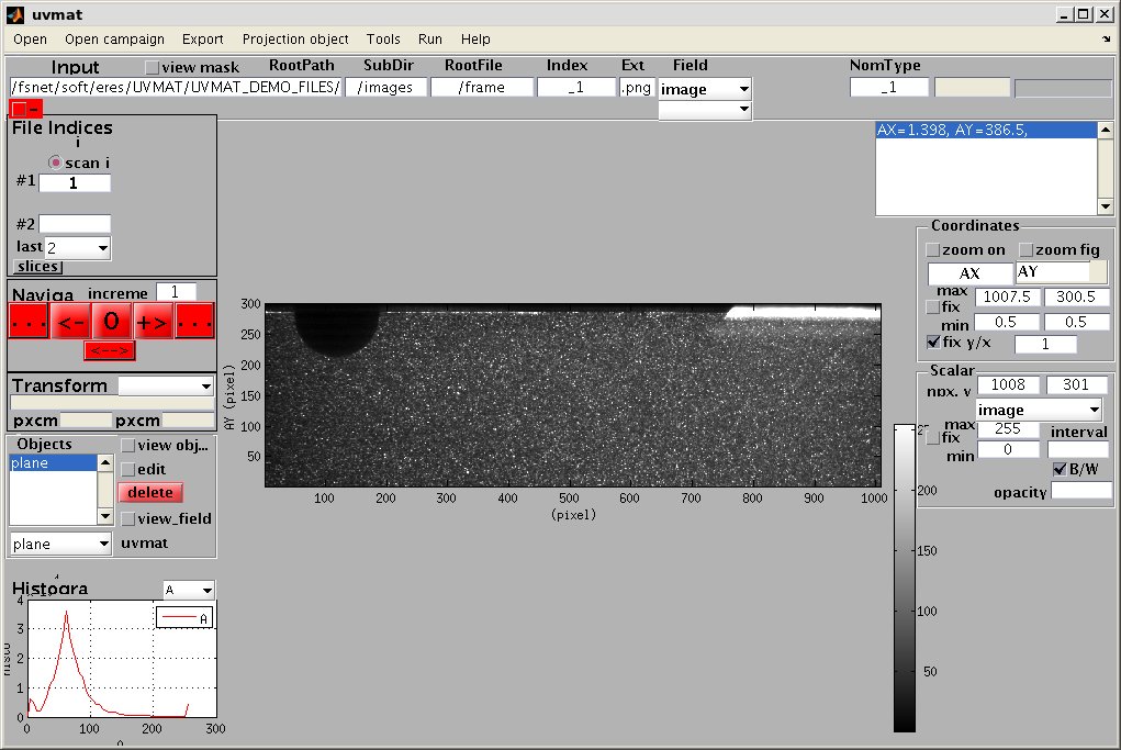
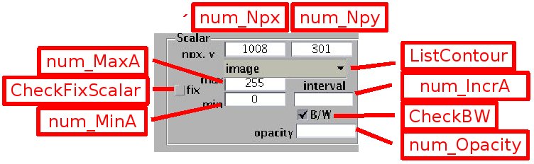
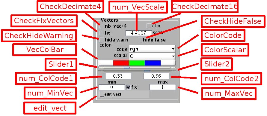
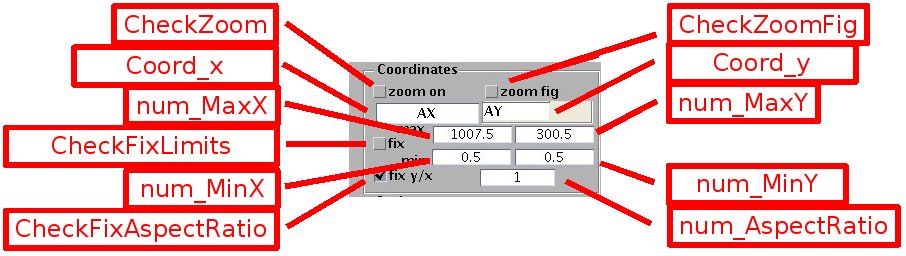
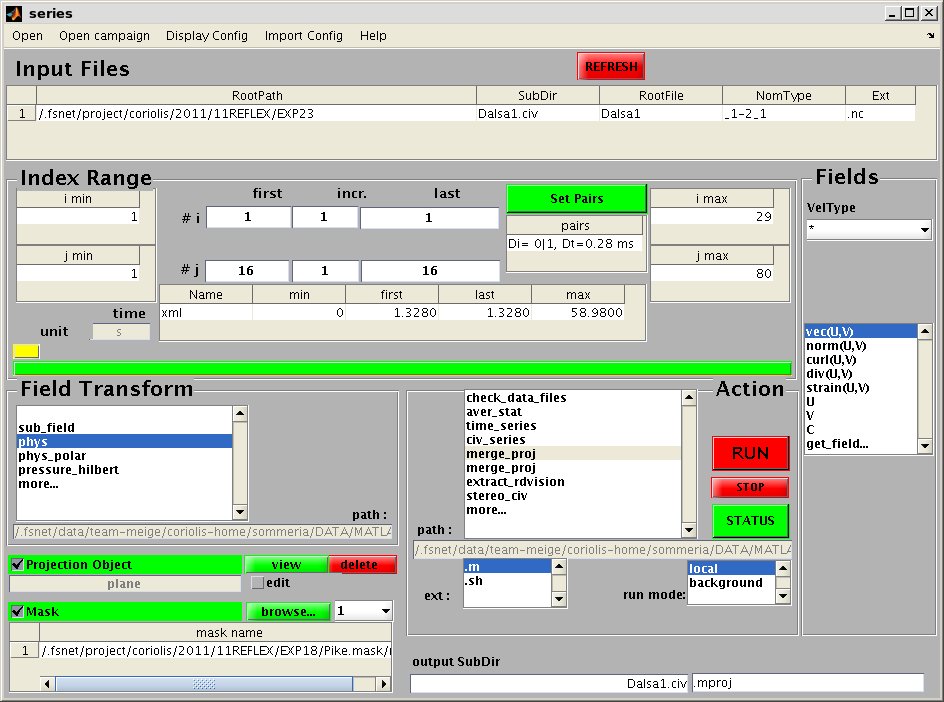
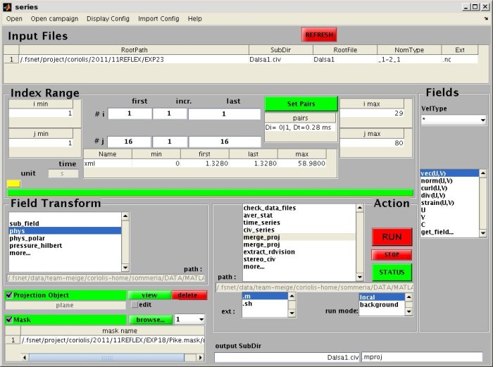
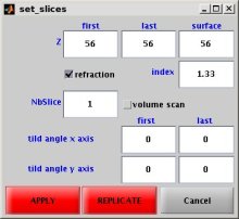
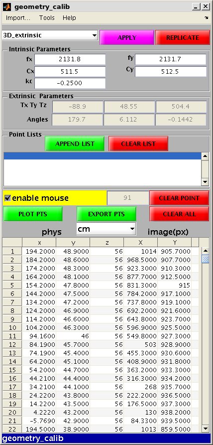
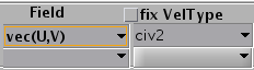
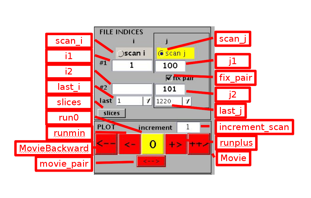
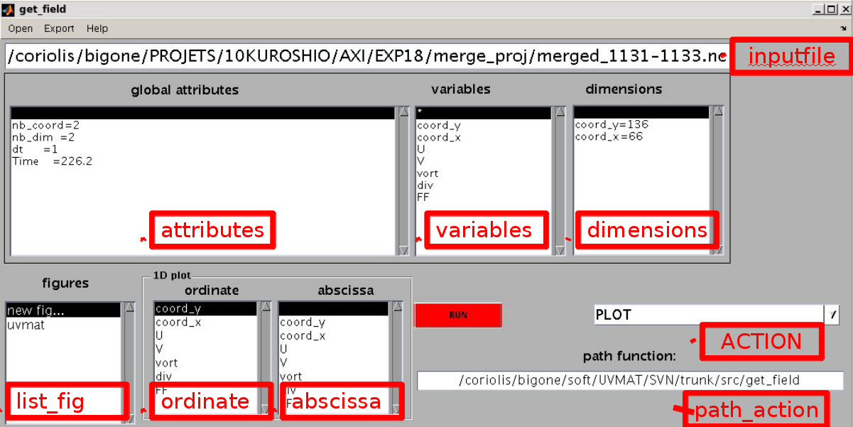
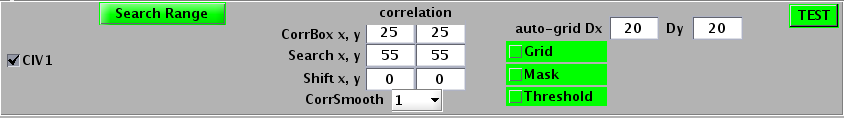
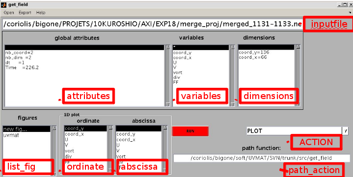
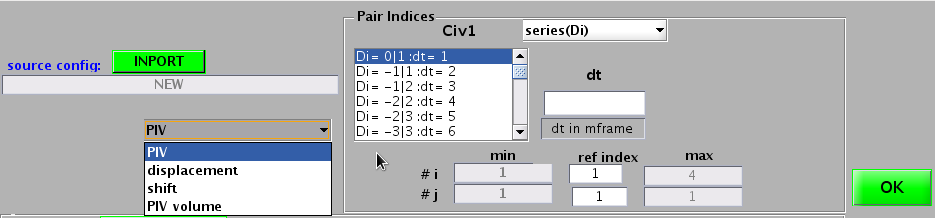
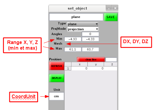
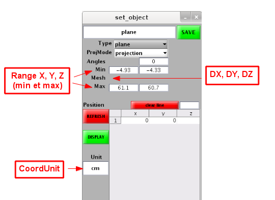
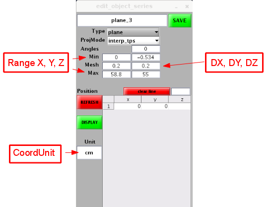
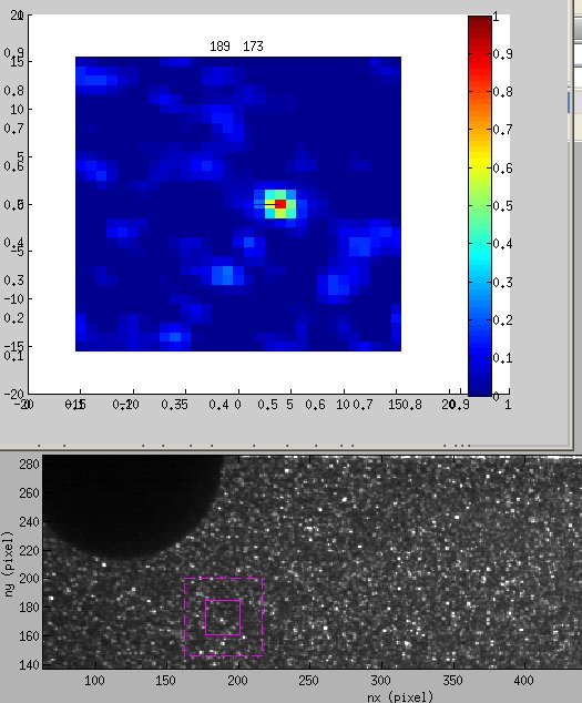
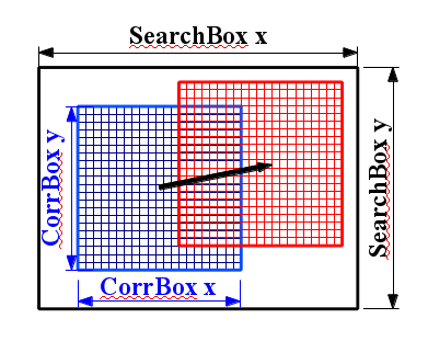
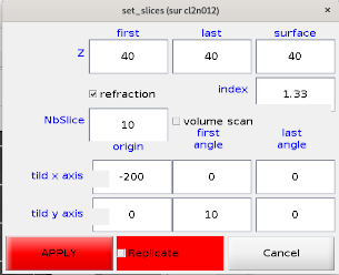
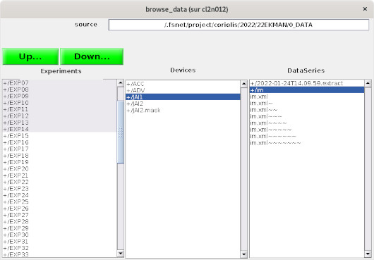