CREST
| Infrastructure | CNRS_Coriolis |
| Project (long title) | Coriolis and Rotational effects on Stratified Turbulence |
| Campaign Title (name data folder) | 16CREST |
| Lead Author | Jeffrey Peakall |
| Contributor | Stephen Darby, Robert Michael Dorrell, Shahrzad Davarpanah Jazi, Gareth Mark Keevil, Jeffrey Peakall, Anna Wåhlin, Mathew Graeme Wells, Joel Sommeria, Samuel Viboud |
| Date Campaign Start | 12/09/2016 |
| Date Campaign End | 21/10/2016 |
0 - Publications, reports from the project
1 - Objectives
Our primary objective is to measure detailed turbulence distributions within channelised gravity currents, as a function of Coriolis forces, concentrating on: i) the bottom boundary layer, ii) redistribution of turbulence within bends, and, iii) redistribution of turbulence at the interface between the gravity current and the ambient. These datasets will enable existing theory on the presence and influence of Ekman boundary layers to be tested, with important implication for the basal shear stress distributions, erosion, and the evolution of channels. These data on the distribution of turbulence will then be applied to i) examine the turbulence distribution in straight channels, ii) provide an analysis of secondary flow and associated turbulence around bends for the first time, and an assessment of how channelized flows alter as a function of Rossby numbers and therefore latitude, iii) assess how the morphodynamics of submarine channels vary as a function of the Rossby number, iv) explain the observed patterns of submarine channel sinuosity with latitude (Peakall et al., 2012; Cossu and Wells, 2013; Cossu et al., 2015), and, v) incorporate the entrainment data into numerical models of submarine channels, in order to address the unanswered question of how these flows traverse such large-distances across very low-angle slopes (Dorrell et al., 2014).
2 - Experimental setup:

2.1 General description
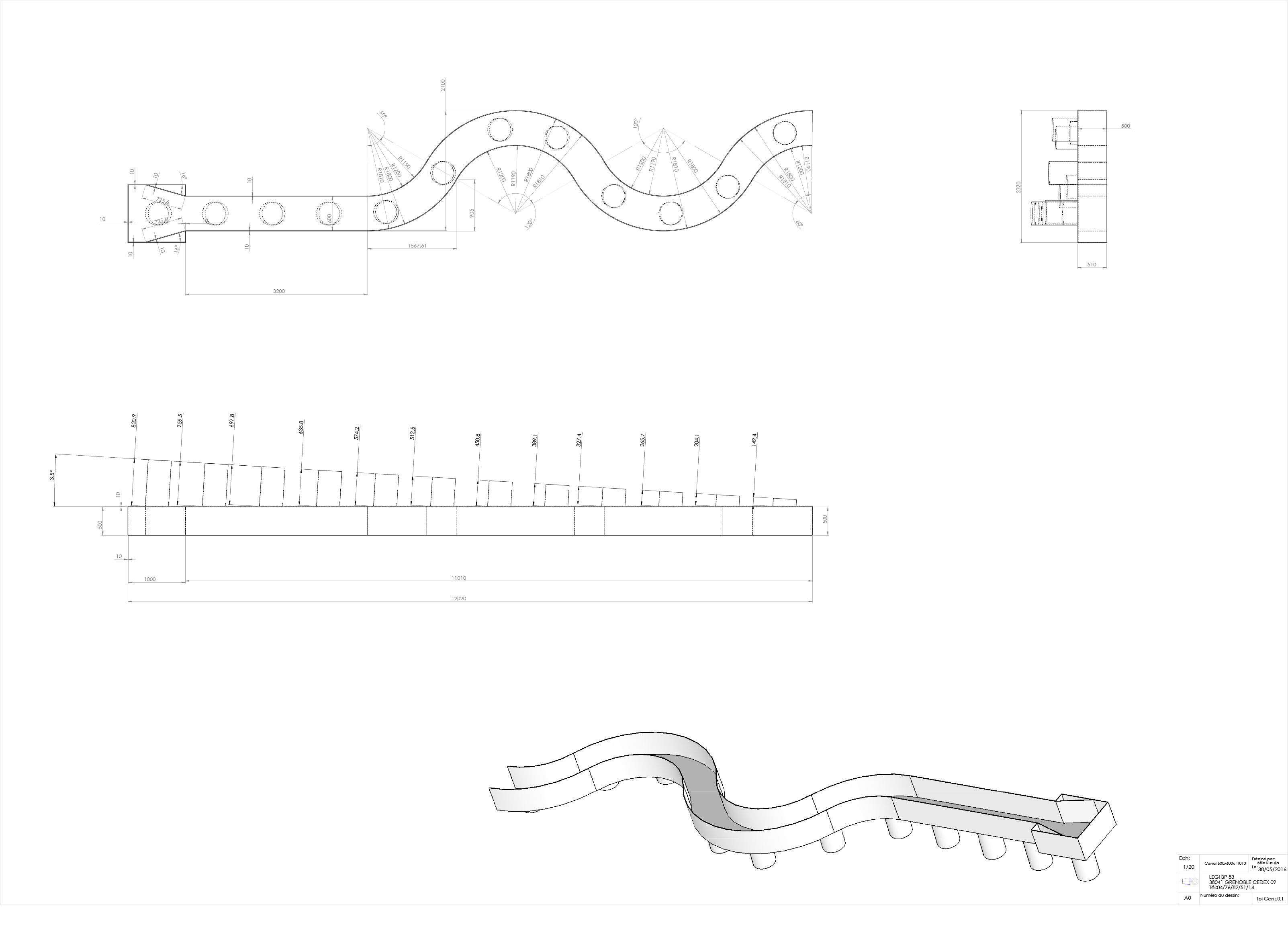
A channel model is positioned within the Coriolis facility. The channel model consists of an initial tapered input section with a honeycomb baffle for flow straightening and turbulence control, a 3.2 m straight channel section, and two bends with a mid-channel radius of 1.5 m. The channel is made of acrylic and is 60 cm wide and 50 cm high; the sinuous section has a sinuosity of 1.2. The slope is 3/50 radians (3.5 degrees, 6% gradient) and the channel terminates 10 cm off of the floor. Saline fluid is pumped into the top of the channel, forming a gravity current, which flows along the channel, and off the end. The basal 10 cm of the flume operates as a sump for the denser saline fluid to accumulate. In turn, this fluid can be drawn down in one of two ways: i) whilst recirculating the fluid, though this is limited to 20 $m3$/hr (5.55 l/s), and ii) through emptying to the drain, in which case any flow rate is possible. Two long metal rails are positioned to either side of the channel model across the full width of the flume. These carry a computerized gantry, which can be positioned at any point along the channel. The gantry itself contains the controls for two Schneider slides, one orientated transverse to the model, and the other connected slide, orientated in the vertical. Thus the system enables xyz control.
2.2 Definition of the co-ordinate system
The co-ordinate system is defined as follows. X is defined as zero at a position 56 cm upstream from the downstream end of the straight channel. This is the position that the basal ADV probe (ADV1) is located at when the traverse is at position X1. Position X4 (at the apex of bend 2) is 7.01 m downstream of position X1.
For ADV the Y-direction is defined relative to the local channel cross-section at any given X-position. The zero position is defined as the right bank of the channel, as looking downstream. The z-position is defined locally from the bed of the channel, for any given XY position, with zero representing the bed.
For PIV the y coordinate is transverse to the channel in the straight part, with origin on the inner right hand side of the channel (looking downstream). The z coordinate is vertical upward with origin at the tank bottom.
The channel system is positioned relative to the centre of the Coriolis table as follows. The centre of the Coriolis table is 13 cm upstream and 45.5 cm to the right hand side (as looking downstream) of the inner bend wall apex position of the first bend [all measurements are taken from the outer edge of the channel wall].
2.3 Fixed Parameters
| Notation | Definition | Values | Remarks |
| $Q_0$ | Input Discharge | $6 \ ls-1$ | |
| $\Delta\rho$ | Input Density Difference | $20 \ kg \ m-3$ | Input box mixing reduces this to approx. $10 \ kg \ m-3$ depth averaged |
| $W$ | Channel Width | $0.6 \ m$ | |
| $\nu$ | Viscosity | $10-6m2s-1$ | |
| $S$ | Slope | $3.5{\circ}$ |
2.4 Variable Parameters
| Notation | Definition | Unit | Initial Estimated Values | Remarks |
| $\Omega$ | Rotation Rate | $rads-1$ | -0.18 - 0.15 | |
| $H_w$ | Water Depth | $m$ | 1-1.1 | |
| $Q_o_u_t_p_u_t$ | Output Flow Rate | $ls-1$ | 5.5 - 17 | |
| $k$ | Roughness | - | - |
2.5 Additional Parameters
| Notation | Definition | Unit | Initial Estimated Values |
| $h$ | Depth of gravity current | $m$ | 0.2-0.4 |
| $U$ | Mean downslope velocity | $ms-1$ | 0.1-0.15 |
| $\delta$ | Thickness of Ekman boundary layer | $mm$ | ~10 |
| $R$ | Centreline radius of curvature | $m$ | 1.5 |
2.6 Definition of the relevant non-dimensional numbers
Flow Reynolds number across the obstruction, $Re = Uh/\nu$.
Densimetric Froude number, $Fr = U/(g'h){1/2}$, $g' = g(\Delta\rho)/\rho_0$.
Rossby number (width), $Ro_W = U/fW$.
Rossby number (radius of curvature), $Ro_R = U/fR$
Canyon number, $\beta = sW/\delta$.
Bulk Richardson number, $Ri = 1/(Fr{2})$
Keulegan number, $Ke = (Ri/Re?){1/3}$
3 - Instrumentation and data acquisition
3.1 Instruments
Two ultrasonic systems are used to measure velocity.
Ultrasonic Velocimetry Profiling (UVP) Ultrasonic velocimetry profiling (UVP) is a technique that measures a single component of velocity at up to several hundred points along a line. A transducer sends out an ultrasonic pulse, and then gates the return signal into a series of spatial bins. The individual transducers can be multiplexed in order to provide pseudo-velocity fields. The transducers are linked via a multiplexer with a delay of 15 ms, so the two-dimensional velocity field is not instantaneous, however velocity fields can be collected at 3-4 Hz. A UVP-duo was used, with two different frequencies of transducers. An array of ten 4 MHz UVP probes (with 10 m long cables) was used for collecting downstream velocity profiles. Initial test experiments used probes positioned at heights of (centre point of each probe): 7, 16, 26, 56, 86, 116, 146, 176, 206 and 236 mm. The actual experiments used probes positioned at heights (centre point of each probe) of 10, 25, 50, 75, 100, 150, 200, 250, 350 and 450 mm from the base of the channel. These probes are positioned in a custom made plastic holder, in turn connected to a bar strapped to the channel top. Initially, the probes are positioned on the channel centreline, 80 mm downstream of the apex of bend 2, looking upstream. An array of ten 2 MHz UVP probes (with 4 m long cables) is used to examine the nature of secondary flow at the second bend apex. This involves drilling holes in the apex of bend 2 and inserting the UVP probes. The probes are positioned at heights of 45, 90, 135, 180, 225, 270, 315, 360, 404, and 450 mm from the base. 2 MHz probes are required for the cross-section measurements since the measurement range needs to be much larger (60 cm) than is required for the axial velocity measurements.
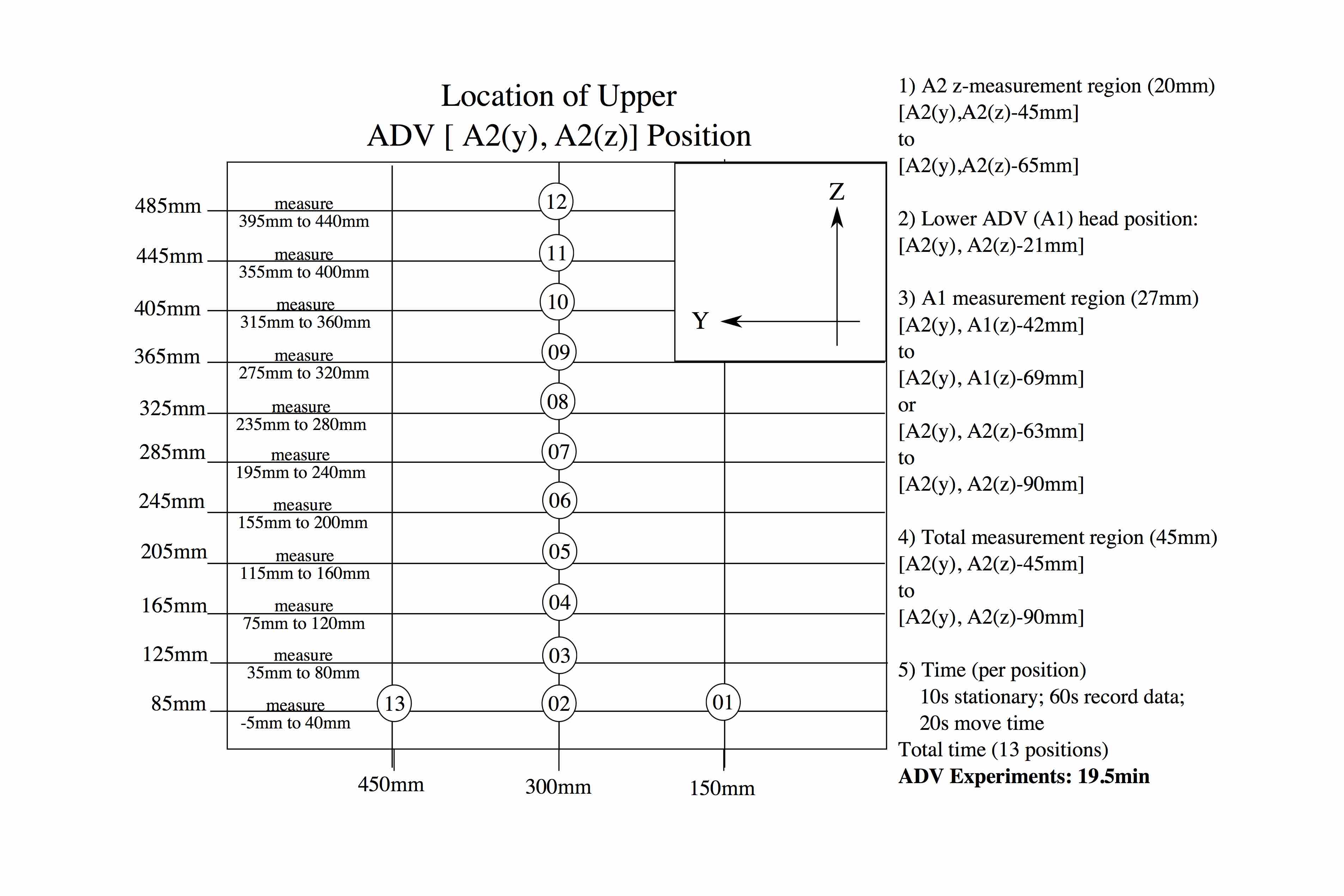
Profiling Acoustic Doppler Velocimetry (ADV) Early experiments used 3 co-mounted Nortek Vectrino Profiler Acoustic Doppler Velocimetry (ADV) probes ADVs for mapping three-dimensional flow velocities, whilst later experiments including the main experiments used 2 ADVs to minimize side lobe interference, and because of the loss of one probe. The ADVs were run at 100Hz in all experiments, both in the initial tests and in the actual experiments. The ADV probes measure three component velocities over a depth range of around 30 mm (up to 34 mm), with this zone starting 40 mm below the probe head. Bottom tracking by the instruments enables this depth to be precisely known and controlled, provided sufficient seeding is present in the flow. ADV collection was fully synchronised with the traverse through sending of the required voltage offset signal to them, thus enabling individual velocity files to be collected for each probe at each traverse. Movement of these probes on the traverse in the y and z planes allows detailed vertical profiles and flow mapping to be undertaken. Initial test experiments used the 3 probes, 1 was a stem probe with additional shielding, and 2 were flexible probes. The basal probe was numbered 1, middle 2, and upper probe 3, and were at heights of 7.2, 10 and 13 cm respectively. Lateral offset in the x-direction was 8.5 cm between probes 1 (most downstream probe) and 2, and 7.5 cm between probes 2 and 3 (most upstream). The traverse positions for each cross-section were based on probe 2 being positioned directly above the cross-section. These 3 probes were co-mounted on the traverse in order to collectively measure over a height of approximately 6 cm. ADV dwell times varied between 30 and 60 seconds.
In the actual data collection experiments, two ADV probes were used. The basal probe is numbered 1, and the upper probe is numbered 3 [keeping with the earlier experimental protocol]. The traverse positions are based on the position of ADV1, the basal and most downstream ADV. The offset in the x-direction is 11 cm between probe 1 (most downstream probe) and probe 3 (most upstream) [i.e. when the traverse is positioned in the zero position (56 cm upstream of the end of the straight channel section) then ADV1 is in the zero position, and ADV3 is at -11 cm]. In the Z-direction they are positioned 14 mm apart. The dwell time at each point is 60 seconds. In the initial position the ADVs start 15 cm from the sidewall. Note that in these experiments the conductivity probe is located 7.3 cm downstream from ADV1, and is offset by 5.5 cm such that its initial position is 20.5 cm from the wall. The ADVs are positioned at the following positions from the floor for each of the measurement positions:
| Run Position | ADV1 (Z-distance above floor) | ADV3 (Z-distance above floor) |
| Straight Section X1 | ||
| Y=15 cm | 7.2 cm | 8.6 cm |
| Y=30 cm | 7.2 cm | 8.6 cm |
| Y=45 cm | 7.2 cm | 8.7 cm |
| Apex bend 2 – X4 | ||
| Y=15 cm | 6.8 cm | 8.6 cm |
| Y=30 cm | 6.7 cm | 8.7 cm |
| Y=45 cm | 6.6 cm | 8.0 cm |
These data suggest that there is some small-scale variation in lateral slope in the bend apex region.
See the attached Traverse.pdf file for details of the complete measurement suite for the main experiments for the ADV and also for Conductivity Probe C0 (with appropriate offset - see above).
Siphon rig The siphon rig consists of 12 siphon tubes, each with a nominal internal diameter of 1.6 mm (3.2 mm external diameter), and 15 m in length. The siphons are held in place in the channel section by a plastic holder which is in turn connected to a rod attached to the channel. The siphon rig is positioned 80 mm downstream of the inflection downstream of bend 2, offset laterally 78 mm off-axis from the position of the UVP (on the right hand side as looking downstream). The siphons were initially positioned at heights of 7, 16, 26, 56, 86, 116, 146, 176, 206, 236, 266 and 306 mm from the bed for the initial test experiments. For the main experiments the siphons were positioned at heights of 10, 25, 50, 75, 100, 125, 150, 175, 200, 250, 350 and 450 mm above the bed. The siphon tubes are connected to a 12 head Watson Marlow 2058 peristaltic pump which is run at the highest setting of 90 rpm. Samples are taken when the traverse (with ADVs and conductivity probe) is positioned upstream measuring the straight section. Samples are collected in an array of 12 plastic containers over a 60 second period, starting at 5, 10, 15, 20, 25, 30 and 35 minutes into the experiment (the start of the experiment is defined as that point where the input is steady – see Section 3.2). The transit time of fluid moving through the siphons was measured using dye and was found to be 1 min and 50 seconds, thus we are actually sampling the flow at 3 min 10 s, 8 min 10 s, 13 min 10 s, 18 min 10 s, 23 min 10 s, 28 min 10 s, and 33 min 10 s (for the main experiments). Each plastic container was 3 cm in diameter and were placed inside a plastic template consisting of 12 3.2 cm diameter holes. Average fill depth of the containers in the 1 minute measurement period was 2.6 cm. Samples were subsequently measured for conductivity using an Anton Paar DMA35 Portable Density Meter.
PME Microscale Conductivity and Temperature Instrument (MSCTI) The Microscale Conductivity and Temperature Instrument (MSCTI) is designed to measure the electrical conductivity and temperature of solutions containing conductive ions. This instrument provides two analog outputs, one linearly proportional to the solution conductivity, and one non-linearly proportional to the solution temperature. One probe is positioned on the traverse, alongside the ADVs, whilst a second probe is positioned at the base of the input box, in the centreline, 7.3 cm upstream of the honeycomb (the upstream edge of the honeycomb itself is positioned 10.7 cm upstream of the join between the curved inlet box and the start of the straight section). For the main experiments, the conductivity probe in the channel is located 7.3 cm downstream from ADV1, and is offset by 5.5 cm such that its initial position is 20.5 cm from the wall; it is positioned 4.4 cm from the floor. The second conductivity probe, positioned in the header box, is situated in the middle of the box and is 2 cm above the floor. The MSCTI outputs two continuous voltage signals, one for conductivity and one for temperature, and these are recorded as part of the LVM file [C0 and T0 are conductivity and temperature for the probe on the traverse (though T0 does not work, since that part of the instrument is broken), and C1 and T1 are conductivity and temperature from the probe mounted in the inlet box]. We briefly had a second probe [just C2] in the inlet but this broke when it was damaged by a large input flow. Later files continue to have C2, but these just consist of noise. The probes are calibrated after each draining of the tank. To calibrate, samples of different densities (as measured with the hand-held Anton Paar density meter) are prepared at a given temperature of 21-22C and these are compared to the voltage output for conductivity of each probe. Because the water is so constant in the experiments, around 21-22C then this calibration approach enables a direct correlation between the voltage representing conductivity, and flow density. As such the temperature output from the two probes (note again that T0 is broken) are not required. The effects of temperature are small, a 1 degree C change in temperature for fresh water changes the conductivity by only 2% (see Barron and Ashton, Reagecon Technical Paper). For the test experiments the Conductivity probe was positioned 0.4 cm upstream, and with a lateral offset of 6.1 cm to the left hand side of the channel as looking downstream; it was 4.2 cm above the bed at the lowermost ADV setting.
Particle Imaging Velocimetry (PIV) A Spectra-Physics Millennia ProS 6W YAG continuous laser (532 nm) in conjunction with 3 cameras was used to provide PIV images. The laser light sheet was brought in parallel to the floor of the channel. The light sheet can then be racked in the vertical through a series of steps through the use of a motorized traverse (tilted at 3.5 degrees to match the slope of the channel) and a mirror set at 45 degrees. The laser has another set of optics to point the light sheet down at the mirror, producing the light sheet. There is a glass window that enables the laser beam to go through the surface of the water tank. A 3D animation of the laser is in the ‘videos’ subfolder of the Photos folder. The laser light sheet positions are then synchronized with the PIV cameras. The field of view extends from close to the upstream end of the first bend, towards the mid-point of the second bend.
Later experiments used larger seeding particles, 200 micron polystyrene particles for the flow seeding. These work very well for these situations where the measurement area is larger than 2 square metres. The three PIV cameras consist of one Falcon1 camera (Falcon 4M, CMOS 2432*1728 pixels, 10 bits) over the upstream part – with a 35 mm objective lens, PCO2 over the first bend with a 35 mm objective lens, and PCO3 over the most downstream part of the PIV measurement area, which has a 20 mm objective lens. 15 slices in the vertical are taken, each containing 20 images and these are repeated 10 times. Four different times between frames are used, since the velocities were not known a priori and vary as a function of height in the gravity current. So as such, no specific frame rate is used. All this is in the .xml files which can be read by a text editor. The two PCO cameras are PCO.edge5.5 CMOS cameras (2560*2160 pixels). The general approach is to have the lowest slice at approximately 2 cm above the floor, and then there are 2.5 cm heights between each successive level. These varied over time however, so there are a number of slightly different setups – see below. The sequence starts at the highest point, and then steps down through the flow, to the bottom, before switching back to the top again. Heights of laser slices (22/09/16 – 2.5 cm but after that 12/10/2016 and 14/10/2016 and 19/10/2016 all at basal 2 cm).
3.2 Definition of time origin and instrument synchronisation
This section relates to the main experiments, and not the test experiments (see diary entries for details of earlier experiments). Conductivity as measured in the inlet box (Probe C1) is seen to vary initially due to mixing within the input box, and because a higher input rate is used in the first minute of the experiment (~11-13 L/s in the main experiments – see Section 6) than later in the flow (~6 L/s). This initial pulse is intended to help to clear fluid out of the inlet box. The time origin is judged to be that point at which the value of this conductivity probe (C1) becomes approximately constant. The timings and synchronisation of the ADV, UVP and the Siphons are controlled with the aid of a stopwatch which is started at the time origin. PIV is then initiated soon after the time origin (approximately 0 minutes) to approximately 10 minutes run time. The timing of PIV initiation can be determined retrospectively, relative to the time origin, because the traverse initiation (that runs the ADV) is specifically linked to the time origin (ADV measurements start at 15 minutes and runs to 35 minutes), and both the traverse and the PIV are tied into the main control software. Thus knowing the time difference between the traverse initiation and the PIV initiation, and subtracting this from 15 minutes provides the PIV initiation relative to the time origin. The UVP and Siphon data are independent as their outputs are not directly tied into the Coriolis control software in the same way that the traverse is. Siphons are initiated after 5 minutes, and the cross-stream UVPs are started at 5 minutes (run until 15 minutes), whilst the downstream UVPs are started at 25 minutes are run until 35 minutes. For 19/10 and 20/10 files the start of the PIV integrates directly with the time origin, all other aspects as before. For PIV analysis, the time origin of the experiment is worked out from the C1 conductivity probe in the input box, where it exhibits the initial sharp rise (near instantaneous) as the flow input starts.
3.3 Requested final output and statistics
Batch processed camera data in to .png files for those experiments from 18-43 that have PIV data, so that images are in a non-proprietary format. PIV analysis of the flow field through multiple horizontal slices in different Z-positions, for the non-rotating case, and for the rotating cases (experiments 18-43 as above), dependent on the quality of the captured PIV images. Average velocity vectors for the channel slices. Potentially information on vorticity would enable the smaller-scale vortical structures that are obvious in some of the videos, to be identified.
4 - Methods of calibration and data processing
The MSCTI conductivity probe is calibrated after each set of experiments when the tank is drained (see Section 3.1 for full details). The ADVs have 4 heads and as such this enables some internal verification of the instrument. The ADV and UVP datasets are processed using a series of bespoke Matlab scripts. The PIV data will be processed using a bespoke script. Access to commercial PIV processing packages is also available.
The images for PIV are calibrated from images of grid put in 0_REF_FILES/Calib_absolu. The 3D calibration involves 'intrinsic parameters' of the optical system obtained from images of the same grid seen with tilt angle (put in /Calib-14-09-3D). Then rotations and translations of the calibration points are introduced to adjust the relationship between image coordinates and physical coordinates defined in section 2.2. See http://servforge.legi.grenoble-inp.fr/projects/soft-uvmat/wiki/UvmatHelp#GeometryCalib for details of the method. The calibration parameters are copied in a xml file beside each image folder with the same name (for instance PCO2.xml for PCO2/). The xml files also containing all the timing information.
All the images and processing results from the images are in the folder 0_PIV under the folder with the name of the experiment.
The images are first extracted from their initial format and written as .png images (compression with no loss of data) labelled by two indices i and j=1 to 20. The index i generally runs from 1 to 150 scanning 15 levels (then coming back to each level 1O times).
A first step in image processing after extraction is to subtract the fixed background and rescale the image intensity leading to a image folder with extension .sback. PIV results are stored as netcdf files (extension .nc) in a folder .sback.civ. These data are still in pixel displacement.
Final velocity data in phys coordinates are stored as 2D matrices under the netcdf format in folders with extension .sback.civ.mproj. They are defined on a physical grid with 1 cm mesh.
5 - Organization of data files
All data related to the project are in:
SERVAUTH4\share\project\coriolis\2016 or
servauth4.legi.grenoble-inp.fr\share\project\coriolis\2016
- 0_DOC: miscellaneous documentation and reports
- 0_MATLAB_FCT: specific matlab functions
- 0_PHOTOS: photos of set-up
- 0_PIV
- Each ‘PIV’ folder contains subfolders for each of the 3 PIV cameras: Dalsa (sometimes Falcon1 – it’s the same thing); PCO2; PCO3 [these are named after the different brands of camera]. Other folders include PCO2.png and PCO3.png which contain processes images of the PCO cameras that are in a non-bespoke format. Other folders that can be within the Camera folder include: Dalsa.sback; Dalsa.sback_1; PCO2.png.civ; PCO2.png.civ_1; PCO2.png.civ_2; PCO2.png.sback: PCO2.png.sback_1; PCO3.png.sback_1. .sback files refer to those files where the background has been subtracted, then civ_1 contains images with the first PIV iteration as processed in UVMAT (Joel’s code) and shows the raw data – with or without the rejected vectors; vectors are shown in four colours, blue = best, green = medium, red = poor, and pink = false. A box can be clicked to hide the false vectors. Civ_2 uses a spline interpretation to interpolate between vectors, so long as they are close enough to the surrounding vectors. Then interpolates all the vectors onto a regular grid. Times for the .png images are in the XML files, or netcdf files.
- 0_Processing: UVP processing scripts in Matlab
- 0_REF_FILES: files of general use (calibration data, grids ...)
- EXP1, EXP2, folder for each experiment with names given in the table below. The names refer to ‘fix’ for non-rotating fixed case, ‘rot’ for rotating case, ‘str1’ for the first straight position (also called position X1), and ‘apex 2’ , for the apex in bend 2 (also referred to as position X4).
- Within each experiments, there is a folder with PIV imagery called ‘Camera’, one for ADV data – ‘ADV’, one for UVP data – ‘UVP’, and one for the data coming directly off of the Coriolis table control system ‘LABVIEW’. Some experiments also contain an ‘Images’ folder or a ‘Gopro folder’ containing Gopro videos.
- Each ‘Camera’ subfolder contains subfolders for each of the 3 PIV cameras: Dalsa (sometimes Falcon1 – it’s the same thing); PCO2; PCO3 [these are named after the different brands of camera]. Other folders include PCO2.png and PCO3.png which contain processes images of the PCO cameras, that are in a non-bespoke format. Other folders that can be within the Camera folder include: Dalsa.sback; Dalsa.sback_1; PCO2.png.civ; PCO2.png.civ_1; PCO2.png.civ_2; PCO2.png.sback: PCO2.png.sback_1; PCO3.png.sback_1
- Each ‘ADV’ subfolder, contains two sub-folders: ‘nkt_files’ containing raw Nortek files, and the ‘mat_files’ are the exported raw data in Matlab format.
- Each ‘UVP’ subfolder contains two folders – one with the experiment name (which is the downstream velocity data) recorded downstream of the velocity inflection downstream of bend apex 2, and one with experiment name ‘_cross’ which contains the cross-stream UVP data recorded at bend apex ‘2. These two folders contain text files for each of the probes. The convention is that Probe 1 is the basal probe, with each subsequent probe being successively higher. There are also .mfprof files which are the raw UVP data in native format. All probes are also integrated into single Matlab files. Lastly, there is a Logfile with the header file for the UVP detailing all of the parameters used in the run.
- Each ‘LABVIEW’ subfolder contains: 1) a .lvm file which is a text file and contains a time-stamp, two voltages for the Conductivity probe on the traverse (C0 – Conductivity, and T0 – temperature [this latter one doesn’t work]), a Trig_cam heading representing the Trigger for the PIV Cameras, Conductivity probe in the input box (C1 and T1), and C2 (this was conductivity for a second probe in the input box which was briefly used before breaking. There is always a record for this but it is just background noise. 2) _position.lvm file which is an XYZ file with a times for the movement of the traverse. 3)Some folders also contain probes.nc files. These are netcdf files and contain the vector data from the processed PIV images.
- Within each experiments, there is a folder with PIV imagery called ‘Camera’, one for ADV data – ‘ADV’, one for UVP data – ‘UVP’, and one for the data coming directly off of the Coriolis table control system ‘LABVIEW’. Some experiments also contain an ‘Images’ folder or a ‘Gopro folder’ containing Gopro videos.
6 - Table of Experiments:
| Experiment No. | Experiment Name | Downstream (x)Position | Density Excess | Input flow | Rotation Rate | Rossby Number | Initial Water Depth | Outflow Rate | Run Time | ADV Dwell Time |
| $(kg \ m-3)$ | $(l \ s-1)$ | $(rad \ s-1)$ | $Ro_W$ | $(m)$ | $(l \ s-1)$ | $(Minutes)$ | $(s)$ | |||
| Test Experiments | ||||||||||
| 0 | fixstr1_1909a | X1 | 20 | 12 | 0 | $\infty$ | 1 | 5.5 | 30 | continuous |
| 1 | fixstr1_2109a | X1 | 10.3 | 12 | 0 | $\infty$ | 1 | 5.5 | 21 | 60 |
| 2 | fixstr1_2109b | X1 | 10.3 | 10 | 0 | $\infty$ | 1 | 5.5 | 21 | 60 |
| 3 | fixstr1_2209a | X1 | 19.2 | 6 to 8 | 0 | $\infty$ | 1 | 5.5 | 21 | 60 |
| 4 | fixstr1_2209b | X1 | 19.2 | 10 | 0 | $\infty$ | 1 | 5.5 | 22 | 60 |
| 5 | fixstr1_2609a | X1 | 19 | 5.9 | 0 | $\infty$ | 1 | 5.5 | 27 | 30 |
| 6 | fixstr1_2609b | X1 | 19 | 5.9 | 0 | $\infty$ | 1 | 5.5 | 30 | 30 |
| 7 | fixstr1_2709a | X1 | 20 | 6 | 0 | $\infty$ | 1 | 5.5 | 20 | 30 |
| 8 | fixstr1_2709b | X1 | 18.4 | 15.3 to 6 | 0 | $\infty$ | 1 | 5.5 | 15 | 30 |
| 9 | fixstr1_2809a | X1 | 20 | 20 to 6 | 0 | $\infty$ | 1 | 5.5 | 15 | 30 |
| 10 | fixapex2_2809b | X4 | 20 | 20 to 6 | 0 | $\infty$ | 1 | 5.5 | 10 | 30 |
| 11 | fixapex2_2809c | X4 | 18.4 | 20 to 6 | 0 | $\infty$ | 1 | 5.5 | 5 | 30 |
| 12 | fixapex2_2809d | X4 | 18.4 | 20 to 6 | 0 | $\infty$ | 1 | 5.5 | 5 | 30 |
| 13 | rotstr1_2909a | X1 | 20.3 | 20 to 5.64 | +0.083 | +1 | 1 | 5.5 | 30 | 30 |
| 14 | rotstr1_2909b | X1 | 20.5 | 20 to 6 | +0.083 | +1 | 1 | 5.5 | 15 | 30 |
| 15 | rotstr1_3009a | X1 | 20.4 | 20 to 5.83 | +0.083 | +1 | 1 | 5.5 | 30 | 30 |
| 16 | rotstr1_3009b | X1 | 20.4 | 20 to 5.5 | +0.083 | +1 | 1 | 5.5 | 35 | 30 |
| 17 | rotstr1_3009c | X1 | 20.4 | 20 to 5.5 | +0.083 | +1 | 1 | 5.5 | 10 | Visualization experiment |
| Main Experiments | ||||||||||
| 18 | fixstr1_0410a | X1 | 18.8 | 13.1 to 5.8 | 0 | $\infty$ | 1 | 5.5 | 36 | 60 |
| 19 | fixapex2_0410b | X4 | 18.8 | 13.1 to 5.8 | 0 | $\infty$ | 1 | 5.5 | 30 | 60 |
| 20 | rotstr1_0510a | X1 | 20 | 13.1 to 5.8 | +0.083 | +1 | 1 | 5.5 | 36 | 60 |
| 21 | rotapex2_0510b | X4 | 18.8 | 13.1 to 5.8 | +0.083 | +1 | 1 | 5.5 | 30 | 60 |
| 22 | rotstr1_0610a | X1 | 20 | 10.97 to 5.75 | +0.167 | +0.5 | 1 | 5.5 | 36 | 60 |
| 23 | rotapex2_0610b | X4 | 19.8 | 10.8 to 5.9 | +0.167 | +0.5 | 1 | 5.5 | 30 | 60 |
| 24 | rotstr1_1010a | X1 | 19.7 | 10.86 to 5.92 | +0.041 | +2 | 1 | 5.5 | 36 | 60 |
| 25 | rotapex2_1010b | X4 | 20.4 | 10.86 to 5.78 | +0.041 | +2 | 1 | 5.5 | 30 | 60 |
| 26 | rotstr1_1010c | X1 | 20.2 | 10.86 to 5.75 | +0.021 | +4 | 1 | 5.5 | 36 | 60 |
| 27 | rotapex2_1010d | X4 | 19.4 | 10.89 to 5.78 | +0.021 | +4 | 1 | 5.5 | 30 | 60 |
| 28 | rotstr1_1210a | X1 | 19.9 | 10.94 to 5.94 | -0.083 | -1 | 1 | 5.5 | 36 | 60 |
| 29 | rotapex2_1210b | X4 | 21.4 | 10.63 to 5.81 | -0.083 | -1 | 1 | 5.5 | 30 | 60 |
| 30 | rotstr1_1310a | X1 | 20.5 | 10.61 to 5.89 | -0.041 | -2 | 1 | 5.5 | 36 | 60 |
| 31 | rotapex2_1310b | X4 | 20.5 | 10.69 to 5.81 | -0.041 | -2 | 1 | 5.5 | 30 | 60 |
| 32 | rotstr1_1310c | X1 | 19.7 | 10.97 to 5.78 | -0.021 | -4 | 1 | 5.5 | 36 | 60 |
| 33 | rotapex2_1310d | X4 | 19.6 | 10.72 to 5.78 | -0.021 | -4 | 1 | 5.5 | 30 | 60 |
| 34 | rotstr1_1410a | X1 | 20.5 | 10.36 to 5.75 | -0.0104 | -8 | 1 | 5.5 | 36 | 60 |
| 35 | rotapex2_1410b | X4 | 20.1 | 10.58 to 5.83 | -0.0104 | -8 | 1 | 5.5 | 30 | 60 |
| 36 | rotstr1_1710a | X1 | 20.1 | 10.61 to 5.83 | -0.0052 | -16 | 1 | 5.5 | 36 | 60 |
| 37 | fixstr1_1810a | X1 | 20.2 | 11.11 to 5.58 | 0 | $\infty$ | 1 | 5.5 | 12 | PIV and UVP and siphon |
| 38 | rotapex2_1810b | X4 | 20.2 | 10.69 to 5.83 | +0.0104 | +8 | 1 | 5.5 | 30 | 60 |
| 39 | rotstr1_1910a | X1 | 20.5 | 10.64 to 5.81 | +0.0104 | +8 | 1 | 5.5 | 36 | 60 |
| 40 | rotapex2_1910b | X4 | 20.1 | 10.92 to 5.81 | -0.0104 | -8 | 1 | 5.5 | 30 | 60 |
| 41 | rotstr1_1910c | X1 | 20.6 | 10.92 to 5.81 | -0.0104 | -8 | 1 | 5.5 | 36 | 60 |
| 42 | rotstr1_2010a | X1 | 20.7 | 10.83 to 5.69 | -0.167 | -0.5 | 1 | 5.5 | 36 | 60 |
| 43 | rotapex2_2010b | X4 | 20.9 | 10.94 to 5.83 | -0.167 | -0.5 | 1 | 5.5 | 30 | 60 |
| 44 | rotstr1_2010c | X1 | 20.8 | 10.94 to 5.83 | -0.167 | -0.5 | 1 | 5.5 | 30 | Visualization experiment |
| 45 | rotstr1_2110b | X1 | 20.5 | 10.69 to 5.89 | -0.083 | -1 | 1 | 5.5 | 30 | Visualization experiment |
7 - Diary:
Monday, September 19th 2016
Experiment name: fixstr1_1909a. Filenames: fixstr1_1909a1, fixstr1_1909a2. Location: Position X1 (75% of the way down the straight section, 56 cm upstream from the end of straight section). Input rate: 12 l/s, density excess: 20 kg/m3. Water was very cloudy to the extent that we were not able to use the laser. No siphon rig was used. Running basal ADV with ADV #1 located 7.2 cm from the base. ADV just measured at one point (no traverse measurement).
Experiment started at 2:45pm and stopped at 3:15 pm. The flow automatically stopped part way through as a valve was not open for recirculating water. Part way through red dye was added to visualise the current. Dye visualisation suggested pretty thin flow on the inner bank and significant super elevation on the outer bank. Some perturbation was observed on the surface of the flow at the outer bank, but otherwise the flow surface appears quite smooth, and mixing appeared to be very low. Mean maximum flow velocity from raw output was around 20 - 25 cm/s. ADV and UVP measured twice, the first is referred to as fixstr1_1909a1 and this had a velocity range of 0.3 m/s on the ADV setting, and 0.25 m/s for the UVP. Instantaneous flow velocities were faster than anticipated, as a result of the steep slope (3.5 degrees) with flow wrapping on both instruments so the velocity range was increased on the ADV and the UVP. A second run period fixstr1_1909a2 had a velocity range of 0.5 m/s on the ADV setting. The UVP setting was 680 mm/s (0.68 m/s).
Tuesday, September 20th 2016
Paint was applied to the tank floor to address a leak in the flume, and the tank floor left to dry and seal. The siphon rig was completed and tested. The laser system was aligned. The position of the basal ADV was refined, Orgasol was required as additional seeding in order for bottom tracking to work effectively. Interesting, the stem (fixed) ADV picks this bottom point up better than the flexible ADV in the absence of seeding. Tested synchronization of ADV with traverse; a problem was identified with the nature of the required input signal. Investigation in progress as to how to address this.
Wednesday, September 21st 2016
Experiment name: fixstr_2109a, b. File names: fixtr1_2109a, fixstr1_2109b. Location: Position X1 (75% down straight section, 56 cm upstream from the end of the straight section). Density excess 10.3 kg/m3.
fixstr1_2109a: The input flow rate was 12 L/s and the total experiment time was 21 minutes. The UVP was turned on as the gravity current entered the inlet box. The ADV was turned on 2 minutes after the UVP saw the flow. Two sets of siphon samples were collected three minutes after the current hit the end of the tank. Sampling was done every 10 minutes: Siphon Set #1 (4:30 to 5:30) and Siphon Set #2 (14:30 to 15:30). The flow was too thick and the velocity was about 18 cm/s. It was speculated that the flow rate should be decreased. Siphon samples showed a density decrease in depth, going from the bottom to the top, and also a decrease over time.
fixstr1_2109b: Since the flow was fast and thick, the flow rate was lowered from 10 L/s (t = 0 to 6 ) to 8 L/s (t = 8 to 13) to 6 L/s (t = 15 to 30). 3 sets of siphon samples were collected for the 3 flow rates at 3 different times (4:55 to 5:55, 12:02 to 13:02, and 19:26 to 20:26). The experiment lasted for 21 minutes.
Thursday, September 22nd 2016
Experiment name: fixstr_2209a, b. File names: fixstr1_2909a, fixstr1_2909b. Location: Position X1 (75% down straight section, 56 cm upstream from the end of the straight section). Density excess 19.2 kg/m3.
Before the experiments samples were collected from the storage tanks which store 10 kg/m3 and 20 kg/m3 salt water in order to check the density. Also, samples from the base and the top of the rotating Coriolis tank were collected. No laser was used since the quality of the water was not good enough.
fixstr1_2909a: Flow rate started with 6 L/s for about 16 minutes. Siphon sample Set #1 was collected around 5 minutes after the start of the experiment for 1 minute. After 7 minutes, a sample was collected from the tank on the third floor where salt water enters from the storage tank. Then the flow rate was increased to 8 L/s. At around 16 minutes constant flow rate was reached and a second set of siphon samples were collected at about 19 minutes for 1 minute deviation. The flow rate then was increased to 10 L/s, but since it took a long time to become constant the UVP stopped. So a second experiment was conducted with a flow rate 10 L/s. Also, the Nikon Camera took 2 videos, 10 minutes each one at the start and one almost right at the end.
fixstr1_2209b: Flow rate was 10 L/s and the total experiment timing was 16 min. The flow rate became constant after about 7 minute, so potentially it was not constant before. One siphon sample was collected at 4:27 for one minute deviation. After measuring the density, it was concluded that the density of the inlet box is much lower than 20 kg/m3 meaning a lot of mixing is occurring there. Therefore, there are two issues that need to be considered for future experiments.
- How to control the density of the inlet box and reduce mixing.
- Start every experiment with a constant flow rate, which takes at least 5 min to occur.
Friday, September 23rd 2016
The tank was drained and cleaned in order to locate, drill and install the 2 Mhz UVPs at the apex of the first curve. The probes were located at 10 points evenly spaced 45 mm apart, starting 45 mm from the bottom. The results from the previous experiments were revised to plan new experiments and updated experimental plan and protocol were provided. A calibration for the conductivity probe on the traverse was plotted. Concentration profiles and plots were updated for the latest experiments. Post-processing of the UVP and ADP data for the conducted experiments were carried out. All of our data on the network was updated including the UVP and ADV.
Monday, September 26th 2016
Experiment name: fixstr1_2609a,b. Filenames: fixstr1_2609a, fixstr1_2609b. Location: Position X1 (75% down straight section, 56 cm upstream from the end of the straight section). Input rate 5.9 l/s. Density excess 19 kg/m3. Laser was not used in the experiments today. Running basal ADV with ADV #1 located 7.2 cm, ADV #2 located at 10 cm and ADV #3 located at 12 cm above channel bed.
fixstr1_2609a: The main goal was to investigate if the concentration of the gravity current, inlet box and tank D were equal (19 kg/m3). The traverse sent one TTL signal to the ADV and didn’t send a return signal so only one measurement at one point was made by the ADVs (all ADVs collected data simultaneously). On the middle ADV (#2) wrapping occurred which indicates that velocity needs to be increased to 0.6 m/s. UVP files showed a fair amount of noise in the data which requires further investigation. We waited about 7:20 minutes for the flow rate to reach a constant value. One person took 6 samples (every 3 minutes, starting at t = 0) from the mixing tank on the third floor which contained the salt water mixture coming from tank D. A second person took 6 samples (every 3 minutes, starting at t = 0) from the inlet box at the upstream end of the channel. A third person took 3 sets of 12 siphon samples every 5 minutes (starting at t = 0, duration = 1 min).
GoPros were installed at three positions as follows: Position 1 - On top of inlet box looking downstream. Position 2 - Inside inlet box focused on inflow pipe. Position 3 - straight section of channel, looking cross-channel. Density measurements of the samples showed that the density in the mixing tank on the third floor and tank D were equal (19 km/m3). However, there was a major decrease of density in the inlet box (max density = 14.8 kg/m3). Density of inlet box needs further investigation.
fixstr1_2609b: Goal was to determine flushing characteristics of the inlet box, and how long it takes to reach steady-state density conditions. Running basal ADV at 5 positions in the bottom cross section only at traverse positions y = 0.016, 0.116, 0.216, 0.316 and 0.416 m (with 5 repetitions). GoPro cameras were mounted at three different positions (Position 1 - Outside rotating tank focused on channel outflow looking upstream. Position 2 - above tank, looking down, focused on bends. Position 3 - straight section of channel, looking cross-channel). Dye was released to visualize the flow. One set of 12 siphon samples (duration = 1 min) was taken 5 minutes after flow rate stabilized. It took 2.5 min for the flow rate to stabilize. The ADV was initialized 5 minutes after flow stabilized. The ADV needed more seeding to improve the signal-to=noise ratio. The GoPro in the inlet box showed a lot of mixing between the current and the ambient which explains the decrease in density in the gravity current in the inlet box. The suggestion was to reduce the inlet box volume to reduce the time to reach steady-state density (by reduce the flushing time).
Tuesday, September 27th 2016
Density of siphon samples from Monday, Sept 26 were measured. Two large PVC tubes (dia ~ 40 cm) were placed in the inlet box and weighted down to reduce the volume (new vol ~ 150 L).
Experiment name: fixstr1_2709a,b. Filenames: fixstr1_2709a, fixstr1_2709b. Location: Position X1 (75% down straight section, 56 cm upstream from the end of the straight section). Input rate 6 l/s. Density excess 20 kg/m3. Laser was not used in the experiments today. Running basal ADV with ADV #1 located 7.2 cm, ADV #2 located at 10 cm and ADV #3 located at 12 cm above channel bed.
Fixstr1_2709a: The goal was to examine the flushing time of the inlet box to see how it behaves once the PVC tubes were installed. One conductivity probe (C1T1) was mounted at the centreline just before the flow straightener (metallic honeycomb). Started with 6 l/s and waited for 5 min to see how inlet box, UVP and pump behaved. The UVP and siphon pump were turned on to fix the suspected pulse that the pump imparted to the UVP. This did not resolve the Signal to Noise Ratio (SNR) issue. The inlet box took a long time to reach a steady conductivity value. It was suggested to start with a higher flow rate and then reduce the flow rate to 6 l/s. The ADV and UVP data were still noisy. No siphon sampling was done.
fixstr1_2709b: It was suggested to install an array of three conductivity probes in a cross-section just before the honeycomb in the inlet box. Only one additional probe was available. As such, two conductivity probes were mounted in the cross section just before the flow straightener (metallic honeycomb): one at the centerline (C2 green) and one 5 cm?? from the right wall (C1T1 black), looking downstream. The traverse was able to move vertically in every cross-section position and the previously outstanding issues have been resolved. Water was initially pumped with a flow rate of 15.28 l/s (55 m3/h). This was the highest achievable flow rate. The water was pumped at this rate for 2 minutes and then reduced to 6 l/s. This seems to achieve the desired effect of reaching a steady conductivity value in a short amount of time in the inlet box. The UVP was set over 10 minutes, but still showed noisy data. No siphon sampling was conducted.
Wednesday, September 28th 2016
Experiment name: fixstr1_2809a and fixapex2_2809b, c, d. Filenames: fixstr1_2809a, fixapex2_2809b, fixapex2_2809c, fixapex_2809d. Location for fixstr1_2809a: Position X1 (75% down straight section, 56 cm upstream from the end of the straight section). Location for fixapex2_2809b, c, d: Position X4 (at the centre of the second apex). Input rate 20 l/s (initial ~2 minutes of each run) then reduced to 6 l/s. Density excess 18.4 kg/m3. Laser was not used in the experiments today. Running basal ADV with ADV #1 located 7.2 cm, ADV #2 located at 10 cm and ADV #3 located at 12 cm above channel bed.
fixstr1_2809a: The goal is to increase the seeding and test the ADVs and UVP for less noise. A new stem ADV was mounted to reduce the noise. The UVP didn’t change in terms of noise issue, so the problem does not lie with the seeding density. Another suggestion was to move the UVP box back to the back bench to reduce interference from the electronics on the traverse. Minimal improvement was seen on the ADV profile. The seeding seems to be getting stuck in the inlet box behind the flow straightening baffles - this was visually observed by a buildup of foam in the inlet box.
fixapex_2809b: The siphons were moved up by 20 cm and the UVP 17 cm. The traverse was also moved to the second apex. The goal for this experiment was to take siphon and UVP data higher than 23.6 cm above the channel bed (previously not possible due to the siphon and UVP configuration), because we want to be able to draw velocity and concentration profiles for 40 cm flow thickness. It was also intended to verify if moving the physical position of the UVP box would impact the data quality. Traverse moved to apex 2 position and siphon samples were taken every 1 minute after flow rate stabilized, for 1 minute sampling time (5-6 min, 7-8 min, 9-10 min). When the flow was released a large cloud of seeding flowed through the channel as a gravity current (presumably seeding caught in inlet box from previous run) and the data on the ADV improved substantially. It was thus concluded that seeding is a viable solution to the noisy data problem (provided a reliable mechanism for seeding the flow, without it getting caught in the inlet box, can be devised). The other suggestion is to increase their distance further apart to avoid side lobe interference. UVP data remained noisy. It is speculated from pressing and GoPro videos that surface waves are produced where the channel sides plunge under the free surface, and that this is the source of the noise in the UVP data.
fixapex_2809c: The goal for this experiment was to turn off the traverse completely then turn on ADV and UVP to check if noise can be reduced. Almost all electronics were turned off on the traverse. Both the UVP and ADV still show a lot of noise. This implies there is either seeding or side lobe effect for the ADV and speculation on surface wave for the UVP.
fixapex_2809d: The new stem ADV was damaged, so the old cable ADV was used instead. Only one experiment was run with just one ADV to see if it will show noise. It didn’t show noise. Since running multiple ADVs showed noise, this means that they are talking to each other. SNR was low, but according to Nortek, in the arms it is still possible to take good data even with low SNR.
Thursday, September 29th 2016
The tank was drained, cleaned, washed, and refilled. The tank was spun with 0.083 rad/s rotation rate (0.8 rpm).
Experiment name: rotstr_2909a, b. Filenames: rotstr1_2909a, rotstr1_2909b. Location: Position X1 (75% down straight section, 56 cm upstream from the end of the straight section). Input rate started from 20 L/s for the first two minutes and then was decreased to 5.64 L/s.
rotstr1_2909a: Density excess was 20.3 kg/m3. Two sets of siphon samples were collected every 5 to 6 minutes and 15 to 16 minutes after the start of experiment. Siphons and UVPs were at the top part of the flow. Gopros took movies from the ping pong balls moving on top of the rotating tank.
rotstr1_2909b: Density contrast was 20.5 kg/m3. Siphons and UVPs were moved down to their original location. Three set of siphon samples were collected every 5 minutes after the start of the experiment. The experiment lasted for 15 minutes.
Friday, September 30th 2016
Experiment name: rotstr1_3009a, b, c. Filenames: rotstr1_3009a, rotstr1_3009b, rotstr1_3009c.
rotstr1_3009a: The total experiment time was 30 minutes. The goal was to use two UVPs and switch between them within the experiment. ADV measurements were collected at the straight section (Position X1 -75% down straight section, 56 cm upstream from the end of the straight section). The stream wise UVP collected data for the first 10 minutes of the experiment. In the second 10 minutes, the UVP was switched to the cross stream and collected data in the cross stream section for the third 10 minutes. It should be noted that the cycle for the cross stream UVP was set to 1500 mistakenly, instead of 666. Bottom check data was collected for both ADVs. Siphon samples were collected every 5 minutes after the flow rate became constant. The 3 sets were sampled at 5 to 6 minutes (Set #1), 15 to 16 minutes (Set #2) and 25 to 26 minutes (Set #3). The laser was used in this experiment.
rotstr1_3009b: The goal was to see how much better the UVP data would be later in the experiment. Input flow rate started from 20 L/s for the first 2 minutes and then was decreased to 5.5 L/s. Density excess and temperature were 20.4 kg/m3 and 23.7 degrees C respectively. The experiment lasted for 35 minutes as opposed to 30 minutes because it was concluded from previous experiments that would show better results later in the experiment. Therefore 5 minutes after the flow rate became constant, the stream wise UVP collected data for 10 minutes. Then, the two UVPs were switched in the next 10 minutes and, finally, the cross stream UVP collected data from 25 to 35 min. A complete sequence of data was collected by the ADV, but it did not restart for some time. Then, it started collecting a second sequence later which was not complete because the experiment ended. The laser did not work in this experiment.
rotstr1_3009c: Input flow rate started from 20 L/s for the first 2 minutes and then was decreased to 5.5 L/s. The goal for this experiment was to add dye and visualize the behaviour of the current at different locations. GoPros? were placed at different locations to take movies of the current and to test which location is the best fit for taking movies.
Monday, October 3rd 2016
The tank was drained, washed and cleaned. New taller probes were built and installed for the stream wise UVP and the siphons. A new sequence for the traverse was considered and calibration for both conductivity probes was completed. All the data and the diary on the Wiki were updated and a new revised experimental plan was proposed for the next three weeks.
Tuesday, October 4th 2016
Test experiments have been completed, and the instrumentation and experimental sequence and conditions optimised. Today, the main data gathering for the experimental programme started. The tank was filled with water. Calibration curves for both probes were prepared (C1 is the conductivity probe in the inlet box and C0 is the one on the traverse). The traverse was reprogrammed for the new sequence. This has been programmed such that the total timing is about 15 minutes, instead of the proposed 19.5 minutes. This was achieved by decreasing the stationary time and the move time, but the ADV dwell time stayed the same (60 s). Two experiments were conducted for Rossby number infinity.
Experiment name: fixstr1_0410a and fixapex2_0410b. File names: fixstr1_0410a, fixapex2_0410b. Density excess and temperature for both experiments were 18.8 kg/m3 and 22.4°C respectively. Input flow rate started with 13.1 L/s and was decreased to 5.8 L/s. The start of the experiments (t=0 on the stopwatch) was when the flow rate and conductivity of the inlet box became constant.
fixstr1_0410a: The total experiment time was 36 minutes. PIV measurements were conducted for the first 10 minutes of the experiment. ADV data was collected at the straight section (Position X1 - 75% down straight section, 56 cm upstream from the end of the straight section) from 15 to 30 min after the flow rate became constant. 7 sets of siphon samples were collected at 5, 10, 15, 20, 25, 30 and 35 minutes after the start of the experiment each with a duration of 1 minute. The cross-stream UVP collected data from 5 to 15 minutes, and the down-stream UVP collected data from 25 to 35 minutes.
fixapex2_0410b: The total experiment time was 30 minutes. ADV measurements were collected from 15 to 30 minutes after the start of the experiment at the second apex (Position X4).
Wednesday, October 5th 2016
The tank was rotated with a rate of 0.083 rad/s (0.8 rpm) in the counter-clockwise direction, which corresponds to a Rossby number of +1. Two experiments were conducted.
Experiment name: rotstr1_0510a and rotapex2_0510b. File names: rotstr1_0510a, rotapex2_0510b. Inflow rate for both runs started with 13.1 L/s and then was decreased to 5.84 L/s until it reached a constant level.
rotstr1_0510a: The total experiment time was 36 mins. PIV measurements were conducted for the first 10 minutes of the experiment. However, the water was not as clear as expected and there were a lot of bubbles on the tank’s wall, so the quality of the PIV data may be low. Density excess and temperature were 20 kg/m3 and 22.6°C, respectively. ADV data were collected at the straight section (Position X1 - 75% down straight section, 56 cm upstream from the end of the straight section) from 15 to 30 min after the flow rate became constant. 7 sets of siphon samples were collected at 5, 10, 15, 20, 25, 30, and 35 minutes after the start of the experiment, with a duration of 1 minute. The cross stream UVP collected data from 5 to 15 minutes, and the down-stream UVP collected data from 25 to 35 minutes.
rotapex2_0510b: The total experiment was 30 minutes. Temperature and density excess were 23°C and 18.8 kg/m3, respectively. ADV measurements were collected from 15 to 30 minutes after the start of the experiment at the second apex (Position X4).
Thursday, October 6th 2016
The tank was rotated with a rate of 0.167 rad/s (1.6 rpm) in the counter-clockwise direction, which corresponds to a Rossby number of +0.5. Two experiments were conducted.
Experiment name: rotstr1_0610a and rotapex2_0610b. File names: rotstr1_0610a, rotapex2_0610b.
rotstr1_0610a: The total experiment time was 36 mins. Inflow rate started with 10.97 L/s and then was decreased to 5.75 L/s until it reached a constant level. The water was dirty so no PIV measurements were conducted. Density excess and temperature were 20 kg/m3 and 22.7°C, respectively. ADV data were collected at the straight section (Position X1 - 75% down straight section, 56 cm upstream from the end of the straight section) from 15 to 30 min after the flow rate became constant. 7 sets of siphon samples were collected at 5, 10, 15, 20, 25, 30, and 35 minutes after the start of the experiment, with a duration of 1 minute. The cross stream UVP collected data from 5 to 15 minutes, and the down-stream UVP collected data from 25 to 35 minutes.
rotapex2_0610b: The total experiment was 30 minutes. Temperature and density excess were 22.4°C and 19.8 kg/m3, respectively. Inflow rate started with 10.8 L/s and then was decreased to 5.9 L/s until it reached a constant level. ADV measurements were collected from 15 to 30 minutes after the start of the experiment at the second apex (Position X4).
Friday, October 7th 2016
The tank was drained, washed and cleaned. Then it was filled and rotated with 0.041 rad/s (0.4 rpm) corresponding to Rossby number of +2. Wiki notes were prepared and the website was updated. All files on the LEGI network were also updated.
Monday, October 10th 2016
Experiment name: rotstr1_1010a, rotapex2_1010b, rotstr1_1010c, rotapex2_1010d. File names: rotstr1_1010a, rotapex2_1010b, rotstr1_1010c, rotapex2_1010d.
Four experiments were conducted. For the first two experiments the tank was rotated with a rate of 0.041 rad/s (0.4 rpm) in the counter-clockwise direction, which corresponds to a Rossby number of +2.
rotstr1_1010a: The total experiment time was 36 mins. Inflow rate started with 10.86 L/s and then was decreased to 5.92 L/s until it reached a constant level. The water was dirty so no PIV measurements were conducted. Density excess and temperature were 19.7 kg/m3 and 23.3°C, respectively. ADV data were collected at the straight section (Position X1 - 75% down straight section, 56 cm upstream from the end of the straight section) from 15 to 30 min after the flow rate became constant. 7 sets of siphon samples were collected at 5, 10, 15, 20, 25, 30, and 35 minutes after the start of the experiment, with duration of 1 minute. The cross stream UVP collected data from 5 to 15 minutes, and the down-stream UVP collected data from 25 to 35 minutes.
rotapex2_1010b: The total experiment was 30 minutes. Temperature and density excess were 23.8°C and 20.4 kg/m3, respectively. Inflow rate started with 10.86 L/s and then was decreased to 5.78 L/s until it reached a constant level. ADV measurements were collected from 15 to 30 minutes after the start of the experiment at the second apex (Position X4).
For the second two experiments the tank was rotated with a rate of 0.021 rad/s (0.2 rpm) in the counter-clockwise direction, which corresponds to a Rossby number of +4.
rotstr1_1010c: The total experiment time was 36 mins. Inflow rate started with 10.86 L/s and then was decreased to 5.75 L/s until it reached a constant level. The water was dirty so no PIV measurements were conducted. Density excess and temperature were 20.2 kg/m3 and 24.3°C, respectively. ADV data were collected at the straight section (Position X1 - 75% down straight section, 56 cm upstream from the end of the straight section) from 15 to 30 min after the flow rate became constant. 7 sets of siphon samples were collected at 5, 10, 15, 20, 25, 30, and 35 minutes after the start of the experiment, with duration of 1 minute. The cross stream UVP collected data from 5 to 15 minutes, and the down-stream UVP collected data from 25 to 35 minutes.
rotapex2_1010d: The total experiment was 30 minutes. Temperature and density excess were 24.1°C and 19.4 kg/m3, respectively. Inflow rate started with 10.89 L/s and then was decreased to 5.78 L/s until it reached a constant level. ADV measurements were collected from 15 to 30 minutes after the start of the experiment at the second apex (Position X4).
Tuesday, October 11th 2016
The tank was drained, washed and cleaned very carefully. Density measurements of siphon samples from previous experiment were done. A revised experimental plan was prepared based on the conducted experiments so far and all the data on the network was updated to the latest experiment. Fresh water is being prepared (heated up) for new experiments tomorrow.
Wednesday, October 12th 2016
The tank was filled and simultaneously rotated with a rate of 0.79 rpm in the clockwise direction corresponding to Rossby number -1. Density measurements of siphon samples from previous experiments were made. Two experiments were conducted at the straight section and the 2nd apex respectively.
Experiment name: rotstr1_1210a, rotapex2_1210b. File names: rotstr1_1210a, rotapex2_1210b.
rotstr1_1210a: The total experiment time was 36 mins. Inflow rate started with 10.94 L/s and then was decreased to 5.94 L/s until it reached a constant level. Density excess and temperature were 19.9 kg/m3 and 24°C, respectively. At the start of the experiment large particles were injected for PIV and measurements were collected. After PIV measurements were done smaller particles were injected for ADV data collection. ADV data were collected at the straight section (Position X1 - 75% down straight section, 56 cm upstream from the end of the straight section) from 15 to 30 min after the flow rate became constant. 7 sets of siphon samples were collected at 5, 10, 15, 25, 30, and 35 minutes after the start of the experiment, with duration of 1 minute. The cross stream UVP collected data from 5 to 15 minutes, and the down-stream UVP collected data from 25 to 35 minutes. The fire alarm distracted this experiments which cause two issues. First th 4th set of siphon samples (t = 20 min) were not collected and second at the start of the ADV measurement the particles were from PIV and at later time smaller particles were injected.
rotapex2_1210b: The total experiment was 30 minutes. Temperature and density excess were 23.7°C and 21.4 kg/m3, respectively. Inflow rate started with 10.63 L/s and then was decreased to 5.81 L/s until it reached a constant level. ADV measurements were collected from 15 to 30 minutes after the start of the experiment at the second apex (Position X4).
Thursday, October 13th 2016
Experiment name: rotstr1_1310a, rotapex2_1310b, rotstr1_1310c, rotapex2_1310d. File names: rotstr1_1310a, rotapex2_1310b, rotstr1_1310c, rotapex2_1310d.
Four experiments were conducted. For the first two experiments the tank was rotated with a rate of 0.041 rad/s (0.4 rpm) in the clockwise direction, which corresponds to a Rossby number of -2.
rotstr1_1310a: The total experiment time was 36 mins. Inflow rate started with 10.61 L/s and then was decreased to 5.89 L/s until it reached a constant level. PIV measurements were conducted. Density excess and temperature were 20.5 kg/m3 and 23°C, respectively. ADV data were collected at the straight section (Position X1 - 75% down straight section, 56 cm upstream from the end of the straight section) from 15 to 30 min after the flow rate became constant. 7 sets of siphon samples were collected at 5, 10, 15, 20, 25, 30, and 35 minutes after the start of the experiment, with duration of 1 minute. The cross stream UVP collected data from 5 to 15 minutes, and the down-stream UVP collected data from 25 to 30 minutes.
rotapex2_1310b: The total experiment was 30 minutes. Temperature and density excess were 22.5°C and 20.5 kg/m3, respectively. Inflow rate started with 10.69 L/s and then was decreased to 5.81 L/s until it reached a constant level. ADV measurements were collected from 15 to 30 minutes after the start of the experiment at the second apex (Position X4).
For the second two experiments the tank was rotated with a rate of 0.021 rad/s (0.2 rpm) in the clockwise direction, which corresponds to a Rossby number of -4.
rotstr1_1310c: The total experiment time was 36 mins. Inflow rate started with 10.97 L/s and then was decreased to 5.78 L/s until it reached a constant level. PIV measurements were conducted. Density excess and temperature were 19.7 kg/m3 and 22.4°C, respectively. ADV data were collected at the straight section (Position X1 - 75% down straight section, 56 cm upstream from the end of the straight section) from 15 to 30 min after the flow rate became constant. 7 sets of siphon samples were collected at 5, 10, 15, 20, 25, 30, and 35 minutes after the start of the experiment, with duration of 1 minute. The cross stream UVP collected data from 5 to 15 minutes, and the down-stream UVP collected data from 25 to 35 minutes.
rotapex2_1310d: The total experiment was 30 minutes. Temperature and density excess were 22.6°C and 19.6 kg/m3, respectively. Inflow rate started with 10.72 L/s and then was decreased to 5.78 L/s until it reached a constant level. ADV measurements were collected from 15 to 30 minutes after the start of the experiment at the second apex (Position X4).
Friday, October 14th 2016
Density of the previous siphon samples were measured and recorded. Also 3 guests (Bob Ecke Philippe Odier and his PhD student Pauline Husseini) were at Coriolis to visit the site and see the experiments. Two experiments were conducted in which the tank was rotated with a rate of 0.0104 rad/s (0.1 rpm) in the clockwise direction, which corresponds to a Rossby number of -8.
Experiment name: rotstr1_1410a, rotapex2_1410b. File names: rotstr1_1410a, rotapex2_1410b.
rotstr1_1410a: The total experiment time was 36 mins. Inflow rate started with 10.36 L/s and then was decreased to 5.75 L/s until it reached a constant level. PIV measurements were also conducted. Density excess and temperature were 20.5 kg/m3 and 22.3°C, respectively. ADV data were collected at the straight section (Position X1 - 75% down straight section, 56 cm upstream from the end of the straight section) from 15 to 30 min after the flow rate became constant. 7 sets of siphon samples were collected at 5, 10, 15, 20, 25, 30, and 35 minutes after the start of the experiment, with duration of 1 minute. The cross stream UVP collected data from 5 to 15 minutes, and the down-stream UVP collected data from 25 to 35 minutes.
rotapex2_1410b:The total experiment was 30 minutes. Temperature and density excess were 22.4°C and 20.1 kg/m3, respectively. Inflow rate started with 10.58 L/s and then was decreased to 5.83 L/s until it reached a constant level. ADV measurements were collected from 15 to 30 minutes after the start of the experiment at the second apex (Position X4).
Monday, October 17th 2016
Density of the previous siphon samples were measured and recorded. One experiment was conducted in which the tank was rotated with a rate of 0.0052 rad/s (0.05 rpm) in the clockwise direction, which corresponds to a Rossby number of -16.
Experiment name: rotstr1_1710a. File names: rotstr1_1710a. rotstr1_1710a: The total experiment time was 36 mins. Inflow rate started with 10.61 L/s and then was decreased to 5.83 L/s until it reached a constant level. PIV measurements were conducted. Density excess and temperature were 20.1 kg/m3 and 22.3°C, respectively. ADV data were collected at the straight section (Position X1 - 75% down straight section, 56 cm upstream from the end of the straight section) from 15 to 30 min after the flow rate became constant. 7 sets of siphon samples were collected at 5, 10, 15, 20, 25, 30, and 35 minutes after the start of the experiment, with duration of 1 minute. The cross stream UVP collected data from 5 to 15 minutes, and the down-stream UVP collected data from 25 to 35 minutes.
When measuring the density of the siphon samples for this experiment it was revealed that the ambient was too salty in the current experiment and the one conducted on Friday. Therefore, no experiments commenced and the tank was drained immediately. Furthermore, Wiki notes were prepared and the website was updated. All files on the LEGI network were also updated.
Tuesday, October 18th 2016
The tank was washed and cleaned and both conductivity probes were calibrated. Some photos were taken from the position of the ADVs, UVPs and the siphon rig. The tank was then filled and one experiment was conducted with a non-rotating tank, which corresponds to a Rossby number of infinity.
Experiment names: fixstr1_1810a, rotapex2_1810b. File names: fixstr1_1810a, rotapex2_1810b.
fixstr1_1810a: The main goal for this experiment was to collect PIV data and shot a high quality movie from above. The total experiment time was 12 mins. Inflow rate started with 11.11 L/s and then was decreased to 5.58 L/s until it reached a constant level. Density excess and temperature were 20.2 kg/m3 and 21.8°C, respectively. 2 sets of siphon samples were collected at 5 and 10 minutes after the start of the experiment each with duration of 1 minute. The the down-stream UVP also collected data for 10 minutes. The laser sheet was set to be 2 cm above the channel's bottom for shooting the movie. The experiment was synched with PIV data collection.
Then the tank was spun up to the rate of 0.0104 rad/s (0.1 rpm) in the counter-clockwise direction corresponding to Rossby number of +8 and a second experiment was conducted.
rotapex2_1810b: The total experiment was 30 minutes. Temperature and density excess were 21.8°C and 20.2 kg/m3, respectively. Inflow rate started with 10.69 L/s and then was decreased to 5.83 L/s until it reached a constant level. ADV measurements were collected from 15 to 30 minutes after the start of the experiment at the second apex (Position X4).
Wednesday, October 19th 2016
Three experiments were conducted. The first experiment was with rotation rate of 0.0104 rad/s (0.1 rpm) in the counter-clockwise direction, which corresponded to Rossby number +8.
Experiment names: rotstr1_1910a, rotapex2_1910b, rotstr1_1910c. File names: rotstr1_1910a, rotapex2_1910b, rotstr1_1910c.
rotstr1_1910a: The total experiment time was 36 mins. Inflow rate started with 10.64 L/s and then was decreased to 5.81 L/s until it reached a constant level. PIV measurements were conducted, which was synched with the start of the experiment and a Gopro camera captured movie from the top. Density excess and temperature were 20.5 kg/m3 and 22.3°C, respectively. ADV data were collected at the straight section (Position X1 - 75% down straight section, 56 cm upstream from the end of the straight section) from 15 to 30 min after the flow rate became constant. 7 sets of siphon samples were collected at 5, 10, 15, 20, 25, 30, and 35 minutes after the start of the experiment, with duration of 1 minute. The cross stream UVP collected data from 5 to 15 minutes, and the down-stream UVP collected data from 25 to 35 minutes.
Then the tank was spun down, stopped and rotated at the rate of 0.0104 rad/s (0.1 rpm) in the clockwise direction, which corresponds to Rossby number -8 and two experiments were conducted.
rotapex2_1910b: The total experiment was 30 minutes. Temperature and density excess were 22.5 °C and 20.1 kg/m3, respectively. Inflow rate started with 10.92 L/s and then was decreased to 5.81 L/s until it reached a constant level. ADV measurements were collected from 16 to 31 minutes after the start of the experiment at the second apex (Position X4).
rotstr1_1910c:The total experiment time was 36 mins. Inflow rate started with 10.97 L/s and then was decreased to 5.81 L/s until it reached a constant level. PIV measurements were conducted, which was synched with the start of the experiment and a Gopro camera captured movie from the top. Density excess and temperature were 20.6 kg/m3 and 22.4°C, respectively. ADV data were collected at the straight section (Position X1 - 75% down straight section, 56 cm upstream from the end of the straight section) from 15 to 30 min after the flow rate became constant. 7 sets of siphon samples were collected at 5, 10, 15, 20, 25, 30, and 35 minutes after the start of the experiment, with duration of 1 minute. The cross stream UVP collected data from 5 to 15 minutes, and the down-stream UVP collected data from 25 to 35 minutes.
More density measurements of siphon samples were conducted, Wiki notes were prepared and the website was updated. All files on the LEGI network were also updated.
Thursday, October 20th 2016
The tank was rotated at the rate of 0.167 rad/s (1.6 rpm) in the clockwise direction, which corresponds to Rossby number -0.5 and three experiments were conducted. Experiment name: rotstr1_2010a, rotapex2_2010b, rotstr1_2010c. File names: rotstr1_2010a, rotapex2_2010b, rotstr1_2010c.
rotstr1_2010a: The total experiment time was 36 mins. Inflow rate started with 10.83 L/s and then was decreased to 5.69 L/s until it reached a constant level. PIV measurements were conducted which was synched with the start of the experiment and a Gopro camera captured movie from the top. Density excess and temperature were 20.7 kg/m3 and 22.7°C, respectively. ADV data were collected at the straight section (Position X1 - 75% down straight section, 56 cm upstream from the end of the straight section) from 15 to 30 min after the flow rate became constant. 7 sets of siphon samples were collected at 5, 10, 15, 20, 25, 30, and 35 minutes after the start of the experiment, with duration of 1 minute. The cross stream UVP collected data from 5 to 15 minutes, and the down-stream UVP collected data from 25 to 35 minutes.
rotapex2_2010b: The total experiment was 31 minutes. Temperature and density excess were 22.7 °C and 20.9 kg/m3, respectively. Inflow rate started with 10.94 L/s and then was decreased to 5.83 L/s until it reached a constant level. ADV measurements were collected from 16 to 31 minutes after the start of the experiment at the second apex (Position X4).
rotstr1_2010c: The total experiment was 15 minutes. The purpose of the experiment was visualization and movie shoot where rhodamine dye was injected in to the flow. Movies were captured using Gopro cameras.
More density measurements of siphon samples were conducted, Wiki notes were prepared and the website was updated. All files on the LEGI network were also updated.
Friday, October 21st 2016
The tank was rotated at the rate of 0.083 rad/s (0.8 rpm) in the clockwise direction, which corresponds to Rossby number -1 and one experiment was conducted for visualization purposes. Two movies were capture including one with the GoPro? and another with a Nikon which had a filter on its lens to match the laser light sheet. All the instruments were removed from the channel. They were cleaned and packed for return. More Wiki notes were prepared and the website was updated. All files on the LEGI network were also updated.
Attachments (5)
-
section 500x600 lg 11010.PDF (195.7 KB) - added by 10 years ago.
Drawing Model on Table
-
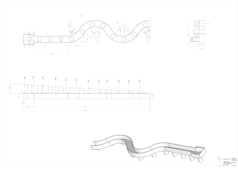
Set_up_drawing.png (212.8 KB) - added by 10 years ago.
Drawing
- Set_up_drawing.jpg (53.9 KB) - added by 10 years ago.
-
Traverse.pdf (46.1 KB) - added by 9 years ago.
Traverse set up for main experiments
-
CRESTTraverseMeasurement.jpg (340.5 KB) - added by 9 years ago.
CREST Traverse Measurement - main experiments
Download all attachments as: .zip