| Version 132 (modified by , 10 years ago) (diff) |
|---|
Project Name
| Infrastructure | CNRS_Coriolis |
| Project (long title) | Coriolis and Rotational effects on Stratified Turbulence |
| Campaign Title (name data folder) | 16CREST |
| Lead Author | Jeffrey Peakall |
| Contributor | Stephen Darby, Robert Michael Dorrell, Shahrzad Davarpanah Jazi, Gareth Mark Keevil, Jeffrey Peakall, Anna Wåhlin, Mathew Graeme Wells, Joel Sommeria, Samuel Viboud |
| Date Campaign Start | 12/09/2016 |
| Date Campaign End | 21/10/2016 |
1 - Objectives
Our primary objective is to measure detailed turbulence distributions within channelised gravity currents, as a function of Coriolis forces, concentrating on: i) the bottom boundary layer, ii) redistribution of turbulence within bends, and, iii) redistribution of turbulence at the interface between the gravity current and the ambient. These datasets will enable existing theory on the presence and influence of Ekman boundary layers to be tested, with important implication for the basal shear stress distributions, erosion, and the evolution of channels. These data on the distribution of turbulence will then be applied to i) examine the turbulence distribution in straight channels, ii) provide an analysis of secondary flow and associated turbulence around bends for the first time, and an assessment of how channelized flows alter as a function of Rossby numbers and therefore latitude, iii) assess how the morphodynamics of submarine channels vary as a function of the Rossby number, iv) explain the observed patterns of submarine channel sinuosity with latitude (Peakall et al., 2012; Cossu and Wells, 2013; Cossu et al., 2015), and, v) incorporate the entrainment data into numerical models of submarine channels, in order to address the unanswered question of how these flows traverse such large-distances across very low-angle slopes (Dorrell et al., 2014).Our primary objective is to measure detailed turbulence distributions within channelised gravity currents, as a function of Coriolis forces, concentrating on: i) the bottom boundary layer, ii) redistribution of turbulence within bends, and, iii) redistribution of turbulence at the interface between the gravity current and the ambient. These datasets will enable existing theory on the presence and influence of Ekman boundary layers to be tested, with important implication for the basal shear stress distributions, erosion, and the evolution of channels. These data on the distribution of turbulence will then be applied to i) examine the turbulence distribution in straight channels, ii) provide an analysis of secondary flow and associated turbulence around bends for the first time, and an assessment of how channelized flows alter as a function of Rossby numbers and therefore latitude, iii) assess how the morphodynamics of submarine channels vary as a function of the Rossby number, iv) explain the observed patterns of submarine channel sinuosity with latitude (Peakall et al., 2012; Cossu and Wells, 2013; Cossu et al., 2015), and, v) incorporate the entrainment data into numerical models of submarine channels, in order to address the unanswered question of how these flows traverse such large-distances across very low-angle slopes (Dorrell et al., 2014).
2 - Experimental setup:

2.1 General description
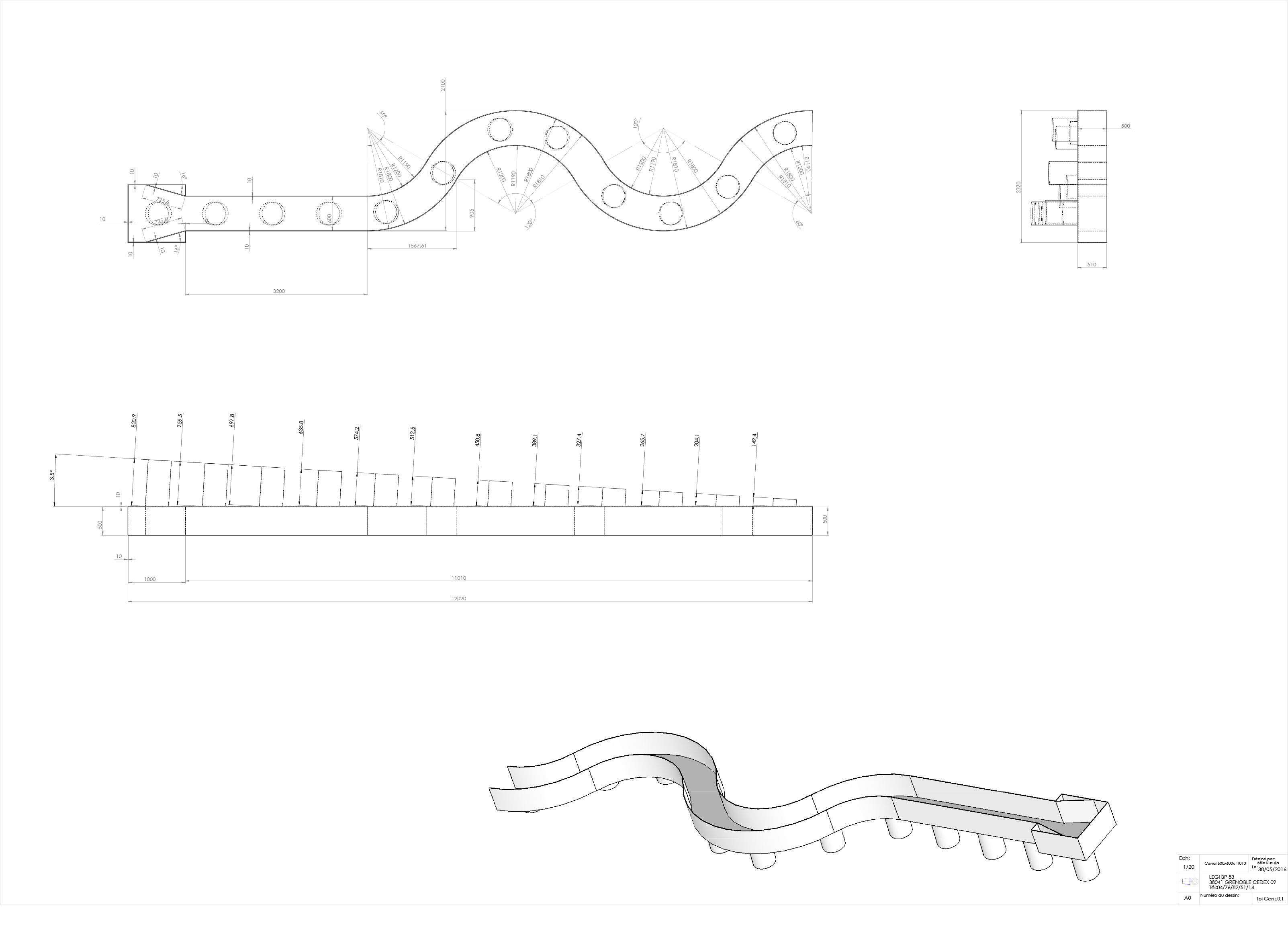
2.1 General description A channel model is positioned within the Coriolis facility. The channel model consists of an initial tapered input section with a honeycomb baffle for flow straightening and turbulence control, a 3.2 m straight channel section, and two bends with a mid-channel radius of 1.5 m. The channel is made of acrylic and is 60 cm wide and 50 cm high; the sinuous section has a sinuosity of 1.2. The slope is 3/50 radians (3.5 degrees, 6% gradient) and the channel terminates 10 cm off of the floor. Saline fluid is pumped into the top of the channel, forming a gravity current, which flows along the channel, and off the end. The basal 10 cm of the flume operates as a sump for the denser saline fluid to accumulate. In turn, this fluid can be drawn down in one of two ways: i) whilst recirculating the fluid, though this is limited to 20 $m3$/hr (5.55 l/s), and ii) through emptying to the drain, in which case any flow rate is possible. Two long metal rails are positioned to either side of the channel model across the full width of the flume. These carry a computerized gantry, which can be positioned at any point along the channel. The gantry itself contains the controls for two Schneider slides, one orientated transverse to the model, and the other connected slide, orientated in the vertical. Thus the system enables xyz control.
2.2 Definition of the co-ordinate system
2.3 Fixed Parameters
| Notation | Definition | Values | Remarks |
| $Q_0$ | Input Density | $12 \ ls-1$ | |
| $\Delta\rho$ | Density Difference | $20 \ kg \ m-3$ | |
| $W$ | Channel Width | $0.6 \ m$ | |
| $\nu$ | Viscosity | $10-6m2s-1$ | |
| $S$ | Slope | $3.5{\circ}$ |
2.4 Variable Parameters
| Notation | Definition | Unit | Initial Estimated Values | Remarks |
| $\Omega$ | Rotation Rate | $rads-1$ | -0.18 - 0.15 | |
| $H_w$ | Water Depth | $m$ | 1-1.1 | |
| $Q_o_u_t_p_u_t$ | Output Flow Rate | $ls-1$ | 5.5 - 17 | |
| $k$ | Roughness | - | - |
2.5 Additional Parameters
| Notation | Definition | Unit | Initial Estimated Values |
| $h$ | Depth of gravity current | $m$ | 0.1 |
| $U$ | Mean downslope velocity | $ms-1$ | 0.1-0.15 |
| $\delta$ | Thickness of Ekman boundary layer | $mm$ | ~10 |
| $R$ | Radius of curvature | $m$ | 1.5 |
2.6 Definition of the relevant non-dimensional numbers
Flow Reynolds number across the obstruction, $Re = Uh/\nu$.
Densimetric Froude number, $Fr = U/(g'h){1/2}$, $g' = g(\Delta\rho)/\rho_0$.
Rossby number, $Ro = U/fW$.
Canyon number, $\beta = sW/\delta$.
Bulk Richardson number, $Ri = 1/(Fr{2})$
Keulegan number, $Ke = (Ri/Re?){1/3}$
3 - Instrumentation and data acquisition
3.1 Instruments
Two ultrasonic systems are used to measure velocity.
Ultrasonic Velocimetry Profiling (UVP) Ultrasonic velocimetry profiling (UVP) is a technique that measures a single component of velocity at either 128 or 256 points along a line. A transducer sends out an ultrasonic pulse, and then gates the return signal into a series of spatial bins. The individual transducers can be multiplexed in order to provide pseudo-velocity fields. The transducers are linked via a multiplexer with a delay of 15 ms, so the two-dimensional velocity field is not instantaneous, however velocity fields can be collected at 3-4 Hz. Two frequencies of transducers will be used. An array of ten 4 MHz UVP probes (with 10 m long cables) will be used for collecting downstream velocity profiles, these probes are positioned at heights (centre point of each probe) of 7, 16, 26, 56, 86, 116, 146, 176, 206 and 236 mm from the base of the channel. These probes are positioned in a custom made plastic holder, in turn connected to a bar strapped to the channel top. Initially, the probes are positioned on the channel centreline, 80 mm downstream of the apex of bend 2, looking upstream. An array of ten 2 MHz UVP probes (with 4 m long cables) will be used to examine the nature of secondary flow at bend apices. This involves drilling holes in the apexes of bends 1 and 2 and inserting the UVP probes. Probes will have to be moved between experiments, to look at the two different bend apexes. 2 MHz probes are required for the cross-section measurements since the measurement range needs to be much larger (60 cm) than is required for the axial velocity measurements.
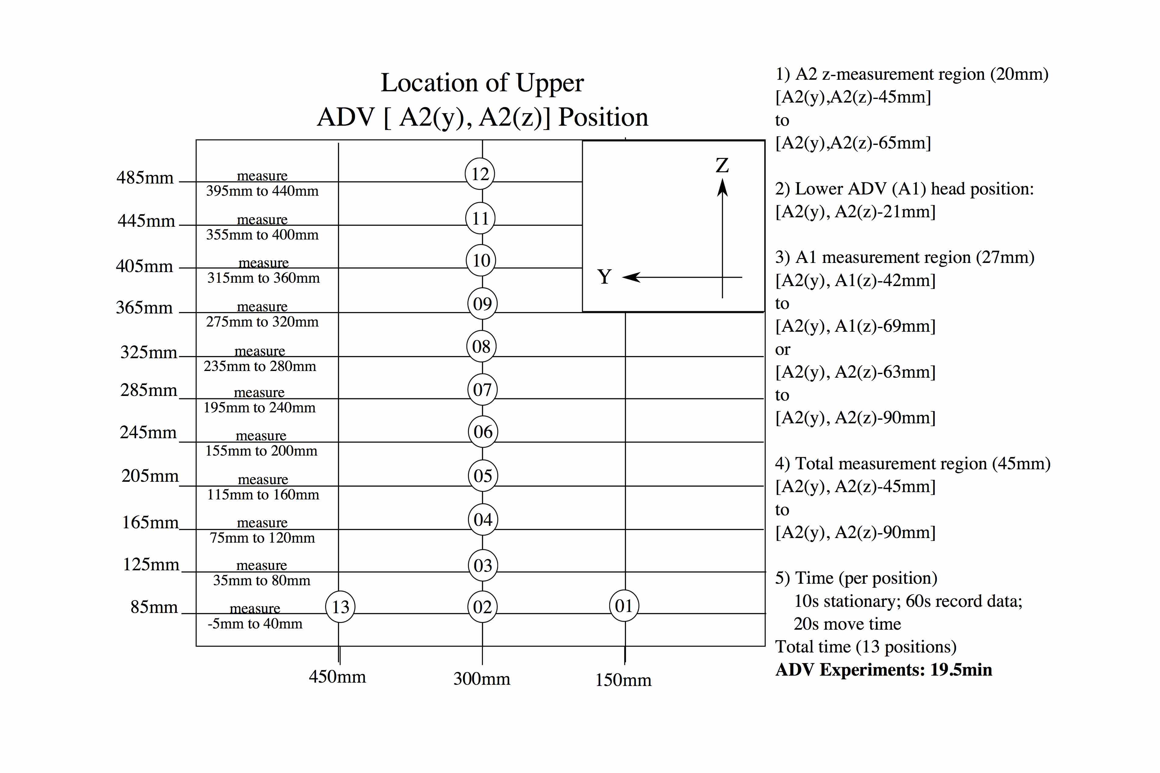
Profiling Acoustic Doppler Velocimetry (ADV) Three profiling Acoustic Doppler probes will be used for mapping three-component flow velocities within the channel. These probes come in two types, 1 is a stem probe with additional shielding, and two are flexible probes that allow closer deployment. All three probes measure three component velocities over a depth range of around 30 mm (up to 34 mm), with this zone starting 40 mm below the probe head. Bottom tracking by the instruments enables this depth to be precisely known and controlled, provided sufficient seeding is present in the flow. These probes are co-mounted on the traverse in order to collectively measure over a height of approximately 6 cm. Movement of these probes on the traverse in the y and z planes allows detailed vertical profiles and flow mapping to be undertaken. Dwell times at each point will vary between 30 and 60 seconds depending on the nature of the experiment. The basal probe is numbered 1, middle 2, and upper probe 3, and are at heights of 7.2, 10 and 13 cm respectively. Lateral offset in the x direction is 8.5 cm between probes 1 (most downstream probe) and 2, and 7.5 cm between probes 2 and 3 (most upstream probe). The traverse positions for each cross-section are based on probe 2 being positioned directly above the cross-section. The aim is to synchronise the ADV collection with the traverse through sending of the required voltage offset signal to them, thus enabling individual velocity files to be collected for each probe at each traverse.
3.2 Definition of time origin and instrument synchronisation
6 - Table of Experiments:
| Run Name | Downstream (x)Position | Density Excess | Input flow | Rotation Rate | Initial Water Depth | Outflow Rate | Run Time | ADV Dwell Time |
| $(kg \ m-3)$ | $(l \ s-1)$ | $(rad \ s-1)$ | $(m)$ | $(l \ s-1)$ | $(Minutes)$ | $(s)$ | ||
| fixstr1_1909a | X1 | 20 | 12 | 0 | 1 | 5.5 | 30 | continuous |
| fixstr1_2109a | X1 | 10.3 | 12 | 0 | 1 | 5.5 | 21 | 60 |
| fixstr1_2109b | X1 | 10.3 | 10 | 0 | 1 | 5.5 | 21 | 60 |
| fixstr1_2209a | X1 | 19.2 | 6 - 8 | 0 | 1 | 5.5 | 21 | 60 |
| fixstr1_2209b | X1 | 19.2 | 10 | 0 | 1 | 5.5 | 22 | 60 |
| fixstr1_2609a | X1 | 19 | 5.9 | 0 | 1 | 5.5 | 27 | 30 |
| fixstr1_2609b | X1 | 19 | 5.9 | 0 | 1 | 5.5 | 30 | 30 |
| fixstr1_2709a | X1 | 20 | 6 | 0 | 1 | 5.5 | 20 | 30 |
| fixstr1_2709b | X1 | 18.4 | 15.3 - 6 | 0 | 1 | 5.5 | 15 | 30 |
| fixstr1_2809a | X1 | 20 | 20 - 6 | 0 | 1 | 5.5 | 15 | 30 |
| fixapex2_2809b | X4 | 20 | 20 - 6 | 0 | 1 | 5.5 | 10 | 30 |
| fixapex2_2809c | X4 | 18.4 | 20 - 6 | 0 | 1 | 5.5 | 5 | 30 |
| fixapex2_2809d | X4 | 18.4 | 20 - 6 | 0 | 1 | 5.5 | 5 | 30 |
7 - Diary:
Monday September 19th 2016
Experiment name: fixstr1_1909a Filenames: fixstr1_1909a1, fixstr1_1909a2 Location: Position X1 (75% of the way down the straight section, 58 cm upstream from the end of straight section). Input rate: 12 l/s, density excess: 20 kg/$m3$. Water was very cloudy to the extent that we were not able to use the laser. No siphon rig was used. Running basal ADV with ADV #1 located 7.2 cm from the base. ADV just measured at one point (no traverse measurement).
Experiment started at 2:45pm and stopped at 3:15 pm. The flow automatically stopped part way through as a valve was not open for recirculating water. Part way through red dye was added to visualise the current. Dye visualisation suggested pretty thin flow on the inner bank and significant super elevation on the outer bank. Some perturbation was observed on the surface of the flow at the outer bank, but otherwise the flow surface appears quite smooth, and mixing appeared to be very low. Mean maximum flow velocity from raw output was around 20 - 25 cm/s. ADV and UVP measured twice, the first is referred to as fixstr1_1909a1 and this had a velocity range of 0.3 m/s on the ADV setting, and 0.25 m/s for the UVP. Instantaneous flow velocities were faster than anticipated, as a result of the steep slope (3.5 degrees) with flow wrapping on both instruments so the velocity range was increased on the ADV and the UVP. A second run period fixstr1_1909a2 had a velocity range of 0.5 m/s on the ADV setting. The UVP setting was 680 mm/s (0.68 m/s).
Tuesday September 20th 2016
Paint was applied to the tank floor to address a leak in the flume, and the tank floor left to dry and seal. The siphon rig was completed and tested. The laser system was aligned. The position of the basal ADV was refined, Orgasol was required as additional seeding in order for bottom tracking to work effectively. Interesting, the stem (fixed) ADV picks this bottom point up better than the flexible ADV in the absence of seeding. Tested synchronization of ADV with traverse; a problem was identified with the nature of the required input signal. Investigation in progress as to how to address this.
Wednesday September 21st 2016
Thursday September 22nd 2016
Friday, September 23rd 2016
The tank was drained and cleaned in order to locate, drill and install the 2 Mhz UVPs at the apex of the first curve. The probes were located at 10 points evenly spaced 45 mm apart, starting 45 mm from the bottom. The results from the previous experiments were revised to plan new experiments and updated experimental plan and protocol were provided. A calibration for the conductivity probe on the traverse was plotted. Concentration profiles and plots were updated for the latest experiments. Post-processing of the UVP and ADP data for the conducted experiments were carried out. All of our data on the network was updated including the UVP and ADV.
Monday, September 26th 2016
Experiment name: fixstr1_2609a,b. Filenames: fixstr1_2609a, fixstr1_2609b. Location: Position X1 (75% down straight section, 58 cm upstream from the end of the straight section). Input rate 5.9 l/s. Density excess 19 kg/m3. Laser was not used in the experiments today. Running basal ADV with ADV #1 located 7.2 cm, ADV #2 located at 10 cm and ADV #3 located at 12 cm above channel bed.
fixstr1_2609a: The main goal was to investigate if the concentration of the gravity current, inlet box and tank D were equal (19 kg/m3). The traverse sent one TTL signal to the ADV and didn’t send a return signal so only one measurement at one point was made by the ADVs (all ADVs collected data simultaneously). On the middle ADV (#2) wrapping occurred which indicates that velocity needs to be increased to 0.6 m/s. UVP files showed a fair amount of noise in the data which requires further investigation. We waited about 7:20 minutes for the flow rate to reach a constant value. One person took 6 samples (every 3 minutes, starting at t = 0) from the mixing tank on the third floor which contained the salt water mixture coming from tank D. A second person took 6 samples (every 3 minutes, starting at t = 0) from the inlet box at the upstream end of the channel. A third person took 3 sets of 12 siphon samples every 5 minutes (starting at t = 0, duration = 1 min).
GoPros were installed at three positions as follows: Position 1 - On top of inlet box looking downstream. Position 2 - Inside inlet box focused on inflow pipe. Position 3 - straight section of channel, looking cross-channel. Density measurements of the samples showed that the density in the mixing tank on the third floor and tank D were equal (19 km/m3). However, there was a major decrease of density in the inlet box (max density = 14.8 kg/m3). Density of inlet box needs further investigation.
fixstr1_2609b: Goal was to determine flushing characteristics of the inlet box, and how long it takes to reach steady-state density conditions. Running basal ADV at 5 positions in the bottom cross section only at traverse positions y = 0.016, 0.116, 0.216, 0.316 and 0.416 m (with 5 repetitions). GoPro cameras were mounted at three different positions (Position 1 - Outside rotating tank focused on channel outflow looking upstream. Position 2 - above tank, looking down, focused on bends. Position 3 - straight section of channel, looking cross-channel). Dye was released to visualize the flow. One set of 12 siphon samples (duration = 1 min) was taken 5 minutes after flow rate stabilized. It took 2.5 min for the flow rate to stabilize. The ADV was initialized 5 minutes after flow stabilized. The ADV needed more seeding to improve the signal-to=noise ratio. The GoPro in the inlet box showed a lot of mixing between the current and the ambient which explains the decrease in density in the gravity current in the inlet box. The suggestion was to reduce the inlet box volume to reduce the time to reach steady-state density (by reduce the flushing time).
Tuesday, September 27th 2016
Density of siphon samples from Monday, Sept 26 were measured. Two large PVC tubes (dia ~ 40 cm) were placed in the inlet box and weighted down to reduce the volume (new vol ~ 150 L).
Experiment name: fixstr1_2709a,b. Filenames: fixstr1_2709a, fixstr1_2709b. Location: Position X1 (75% down straight section, 58 cm upstream from the end of the straight section). Input rate 6 l/s. Density excess 20 kg/m3. Laser was not used in the experiments today. Running basal ADV with ADV #1 located 7.2 cm, ADV #2 located at 10 cm and ADV #3 located at 12 cm above channel bed.
Fixstr1_2709a: The goal was to examine the flushing time of the inlet box to see how it behaves once the PVC tubes were installed. One conductivity probe (C1T1) was mounted at the centerline just before the flow straightener (metallic honeycomb). Started with 6 l/s and waited for 5 min to see how inlet box, UVP and pump behaved. The UVP and siphon pump were turned on to fix the suspected pulse that the pump imparted to the UVP. This did not resolve the SNR issue. The inlet box took a long time to reach a steady conductivity value. It was suggested to start with a higher flow rate and then reduce the flow rate to 6 l/s. The ADV and UVP data were still noisy. No siphon sampling was done.
fixstr1_2709b: It was suggested to install an array of three conductivity probes in a cross-section just before the honeycomb in the inlet box. Only one additional probe was available. As such, two conductivity probes were mounted in the cross section just before the flow straightener (metallic honeycomb): one at the centerline (C2 green) and one 5 cm?? from the right wall (C1T1 black), looking downstream. The traverse was able to move vertically in every cross-section position and the previously outstanding issues have been resolved. Water was initially pumped with a flow rate of 15.28 l/s (55 m3/h). This was the highest achievable flow rate. The water was pumped at this rate for 2 minutes and then reduced to 6 l/s. This seems to achieve the desired effect of reaching a steady conductivity value in a short amount of time in the inlet box. The UVP was set over 10 minutes, but still showed noisy data. No siphon sampling was conducted.
Wednesday, September 28th 2016
Experiment name: fixstr1_2809a and fixapex2_2809b, c, d. Filenames: fixstr1_2809a, fixapex2_2809b, fixapex2_2809c, fixapex_2809d. Location for fixstr1_2809a: Position X1 (75% down straight section, 58 cm upstream from the end of the straight section). Location for fixapex2_2809b, c, d: Position X4 (at the centre of the second apex). Input rate 20 l/s (initial ~ 2 minutes of each run) then reduced to 6 l/s. Density excess 18.4 kg/$m3$. Laser was not used in the experiments today. Running basal ADV with ADV #1 located 7.2 cm, ADV #2 located at 10 cm and ADV #3 located at 12 cm above channel bed.
fixstr1_2809a: The goal is to increase the seeding and test the ADVs and UVP for less noise. A new stem ADV was mounted to reduce the noise. The UVP didn’t change in terms of noise issue, so the problem does not lie with the seeding density. Another suggestion was to move the UVP box back to the back bench to reduce interference from the electronics on the traverse. Minimal improvement was seen on the ADV profile. The seeding seems to be getting stuck in the inlet box behind the flow straightening baffles - this was visually observed by a buildup of foam in the inlet box.
fixapex_2809b: The siphons were moved up by 20 cm and the UVP 17 cm. The traverse was also moved to the second apex. The goal for this experiment was to take siphon and UVP data higher than 23.6 cm above the channel bed (previously not possible due to the siphon and UVP configuration), because we want to be able to draw velocity and concentration profiles fro 40 cm flow thickness. It was also intended to verify if moving the physical position of the UVP box would impact the data quality. Traverse moved to apex 2 position and siphon samples were taken every 1 minute after flow rate stabilized, for 1 minute sampling time (5-6 min, 7-8 min, 9-10 min). When the flow was released a large cloud of seeding flowed through the channel as a gravity current (presumably seeding caught in inlet box from previous run) and the data on the ADV improved substantially. It was thus concluded that seeding is a viable solution to the noisy data problem (provided a reliable mechanism for seeding the flow, without it getting caught in the inlet box, can be devised). The other suggestion is to increase their distance further apart to avoid side lobe interference. UVP data remained noisy. It is speculated from pressing and GoPro videos that surface waves are produced where the channel sides plunge under the free surface, and that this is the source of the noise in the UVP data.
Thursday, September 29th 2016
Friday, September 30th 2016
Attachments (5)
-
section 500x600 lg 11010.PDF (195.7 KB) - added by 10 years ago.
Drawing Model on Table
-
Set_up_drawing.png (212.8 KB) - added by 10 years ago.
Drawing
- Set_up_drawing.jpg (53.9 KB) - added by 10 years ago.
-
Traverse.pdf (46.1 KB) - added by 9 years ago.
Traverse set up for main experiments
-
CRESTTraverseMeasurement.jpg (340.5 KB) - added by 9 years ago.
CREST Traverse Measurement - main experiments
Download all attachments as: .zip