- ICESHELF
- 0 - Publications, reports from the project
- 1 - Objectives
- 2 - Experimental setup:
- 3 - Instrumentation and data acquisition
- 4 - Methods of calibration and data Processing
- 5 - Good to know…
- 6 - Organization of data files
-
7 - Diary for Shelf Break Experiments:
- 7.1 Thursday 07 September
- 7.2 Friday 08 September
- 7.3 Monday 11 September
- 7.4 Tuesday 12 September
- 7.5 Wednesday 13 September
- 7.6 Thursday 14 September
- 7.7 Friday 15 September
- 7.8 Monday 18 September
- 7.9. Tuesday 19 September
- 7.10 Wednesday 20 September
- 7.11 Thursday 21 September
- 7.12 Friday 22 September
- 7.13 Monday 25 September
- 8 - Table with Shelf Break experiments
- 9 - Table with Ice Shelf Experiments
ICESHELF
| Infrastructure | CNRS_Coriolis Topographic Barriers and warm Ocean currents controlling Antarctic ice shelf melt |
| Project (long title) | Topographic Barriers and warm Ocean currents controlling Antarctic ice shelf melt |
| Campaign Title (name data folder) | 17ICESHELF |
| Lead Author | Elin Darelius (part I) and Anna Wåhlin (part II) |
| Contributors | Nadine Steiger, Lucie Vignes,Mirjam Glessmer, Joel Sommeria, Samuel Viboud |
| Date Campaign Start | 04/09/2017 |
| Date Campaign End | 27/10/2017 |
0 - Publications, reports from the project
1 - Objectives
The warm water threatening to melt the Antarctic ice shelves originates from the deep ocean north of the continental shelf. In order for the warm water to reach the ice shelf cavities it has to pass to topographic barriers: the shelf break and the ice shelf front. In a series of experiments we will explore the role of topography in controlling the onshelf flow of warm water.
2 - Experimental setup:
2.1 General description
The two Barriers - the shelf break and the ice shelf front - will be studied in two separate sets of Experiments:
Part I: Shelf break experiments
An idealized topography representing a widening continental shelf and a trough crosscutting the Continental shelf break is used and the effect of changing 1) water depth, 2) radius of curvature, 3) rotation rate and 4) flow speed will be explored. The experiments will be repeated with a) a barotropic and b) a baroclinic (inflow water fresher than ambient water) current.
Part II: Ice shelf experiments
An idealized topography of a v-shaped channel sloping downwards towards an ice shelf front is used. The effect of changing 1) ice shelf draft, 2) ice shelf tilt, 3) rotation rate, and 4) flow speed will be explored. The experiments will be repeated with a) a barotropic and b) a baroclinic (inflow water denser than ambient water) current.
2.2 Topography
2.2.1 Topography for the shelf break experiments

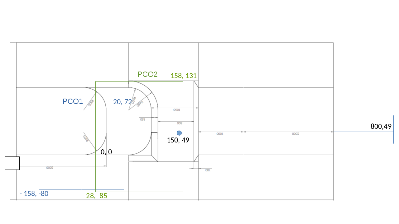
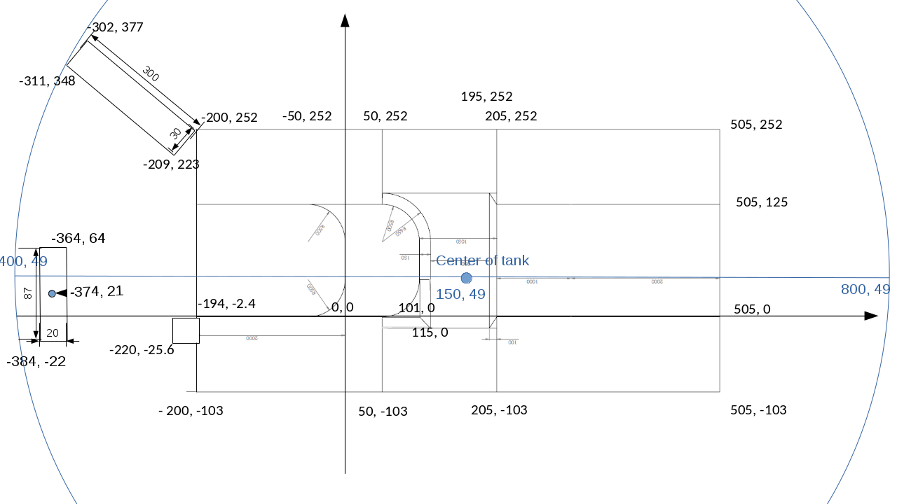
Sketch of the topography of the continental shelf, as well as the skimmer (at - 374,21) to keep the water level constant and a wall (upper left) to prevent the circulating water from disturbing the inflow. View from above with the distances to the (0, 0) coordinate, which is the center of the tank. The blue circle and the blue line are the tank wall and the centerline, respectively.

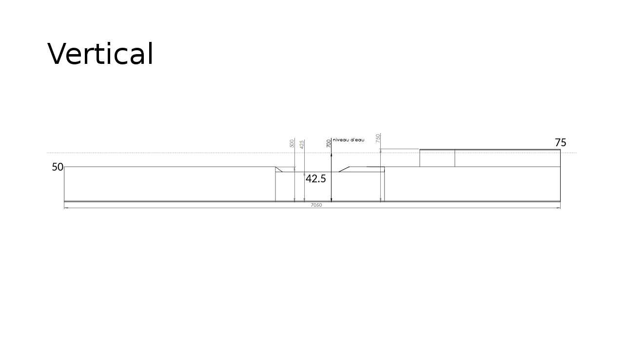
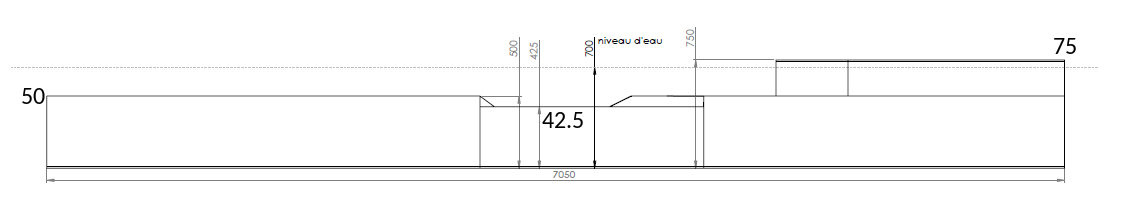
Sketch of the shelf topography seen from the side with the heights of the different areas.
From experiment 18 the source was moved 2.00m further back! The position of the source relative to the topography stayed as before.
2.2.2 Topography for the ice shelf experiments

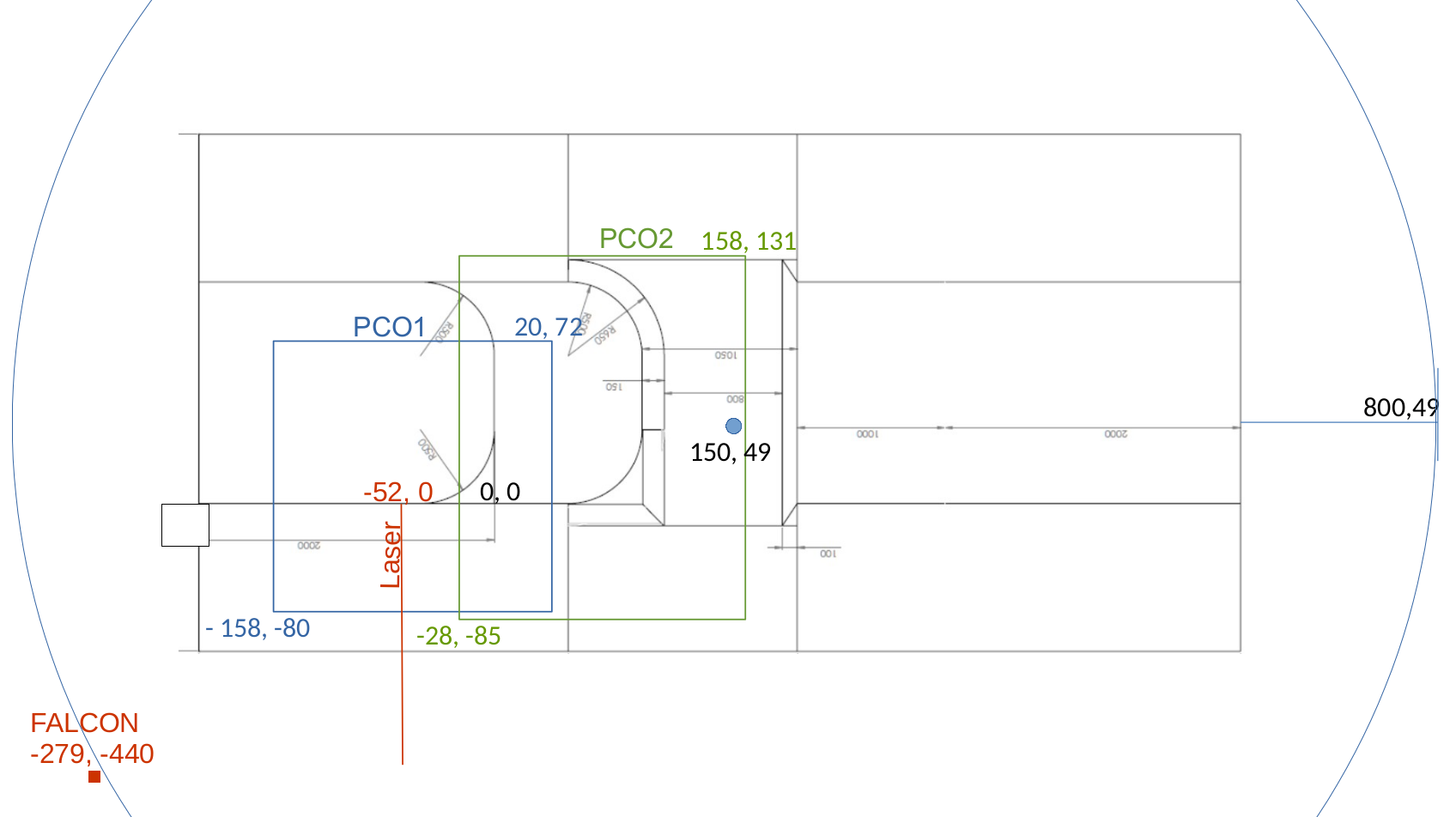
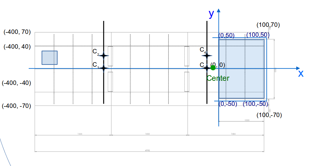
Sketch of the topography of the v-shaped channel seen from above with the distances to the (0, 0) coordinate, which is the center of the tank. The transparent Plexi-glass ice shelf is marked in blue.

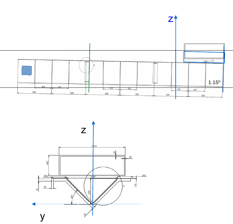
Sketch of the topography of the v-shaped channel and the ice shelf seen from the side including the source in blue and the location of the vertical laser in green, the adjustable ice shelf is marked in blue at the right end of the channel. The lower drawing shows the channel and ice shelf seen from the end into the channel towards the source.
2.3 Reference axis
2.3.1 Reference axis for shelf break experiments
By definition we will use Ox and Oy axis to define the along slope and the cross slope axis. The central reference point (0,0) along the slope is chosen to be the first "land" corner downstream of the source. Positive u - direction corresponds to the along slope flow direction, while positive v - direction is directed onshelf. The position of the topography relative to this coordinate system is shown in 2.2.1
2.3.2 Reference axis for ice front experiments
By definition we will use Ox and Oy axis to define the along channel and cross channel axis. The central reference point (0,0) is chosen to be at the front of the ice shelf and in the middle of the channel. Positive u - direction corresponds to the flow direction towards the ice shelf and positive v - direction is directed to the "west".
2.4 References axis along the wall (horizontal and vertical)
By definition we will use Ox and Oy axis to define the along shore and the cross shore axis. The central reference point (0,0) along the wall is chosen to be the closest point to the center of the tank. Positive direction corresponds to the mean wave or the mean flow direction.
We measure the water level at the wall and in the center of the tank to quantify the impact of the free surface deformation. We also measure the height of the horizontal laser to determine the possible vertical deviation of the laser sheet.

2.5 Parameters for Shelf Break Experiments
2.5.1 Fixed Parameters
| Notation | Definition | Values | Remarks |
| $H_{shelf}$ | Shelf height | 0.5 m | |
| $H_{through}$ | Trough height | 0.42 m | |
| $W_{trough-slope}$ | Width of slope in trough | 10 cm | |
| $s$ | slope in trough | !1:2(Height:Width) | |
| $\nu$ | Viscosity | 10-6 m2 s-1 | |
| $L$ | Total length of the wall | 3 m | |
| $W_{Source}$ | Width of source (inner) | 23 cm |
2.5.2 Variable Parameters
| Notation | Definition | Unit | Initial Estimated Values | Remarks |
| $T_{rotation}$ | Rotation period | s | 30, 50 | |
| $H_{water}$ | Total water depth | cm | 60 - 70 | |
| $H_{shelf}$ | Depth on shelf | cm | 10 - 20 | |
| $R_c$ | Radius of curvature | m | 0 - 0.5 | |
| $Q$ | Flux | L min-1 | 5, 10, 20, 35, 50, 80, 110, 150 | |
| $\Delta \rho$ | Density difference (ambient - inflow) | kg m-1 | 0, 3, 5, 10 |
2.6 Parameters for Shelf Break Experiments
2.6.1 Fixed Parameters
| Notation | Definition | Values | Remarks | |
| $L$ | Channel lengthh | 5 m | ||
| $W$ | Channel width | 1 m | ||
| $H$ | Channel height | 0.5 m | depth of channel center to flanks | |
| $\alpha$ | Slope of channel walls | 45o | ||
| $\beta$ | Slope of channel | 1.15o | ||
| $H_{iceshelf}$ | Ice Shelf thickness | 0.4 m | ||
| $\nu$ | Viscosity | 10-6 m2 s-1 | ||
| $W_{Source}$ | Width of source (inner) | 23 cm | ||
| $H_{water}$ | Total water depth | 90 cm | ||
2.6.2 Variable Parameters
| Notation | Definition | Unit | Initial Estimated Values | Remarks |
| $T_{rotation}$ | Rotation period | s | 30, 60 | |
| $dH_{iceshelf}$ | ice shelf draft | cm | 0, 5, 10, 15, 20, 30, 30-0, 15-0 | 30(15)-0 means tilted ice shelf |
| $Q$ | flow rate | L min-1 | 15,30,50,60 | |
| $\Delta \rho$ | Density difference (ambient - inflow) | kg m-1 | 0,1,2 |
2.7 Definition of the relevant non-dimensional numbers
Rossby number, $ Ro = U/W/f$.
Relative step size, $H* = \delta H/ (H-\delta H) $. (Cenedese et al, 2005)
Depth of baroclinic current ($H_{BC}=sqrt(2Qf/g')$ (Chapman & Lenz 1994; Sutherland et al, 2009)
Internal rossby radius ($\lambda_i = sqrt (g' H_{BC})/f$.
3 - Instrumentation and data acquisition
3.1 Instruments
Conductivity Sondes (CS)
Particle Imaging Velocimetry (PIV) A Spectra-Physics Millennia ProS 6W YAG continuous laser (532 nm) in conjunction with 2 cameras was used to provide PIV images. The laser light sheet was brought in parallel to the bottom of the tank in case of the slope front experiments and tilted by 2% to match the slope of the channel in case of the ice front experiments. The light sheet can then be racked in the vertical through a series of steps through the use of a motorized traverse and a mirror set at 45 degrees. The laser has another set of optics to point the light sheet down at the mirror, producing the light sheet. The laser light sheet positions are then synchronized with the PIV cameras. The laser light sheets cover the whole topography, but are slighlty bended towards the sides, so that they are closer to the bottom at the source and at the end of the topography compared to the middle. Also a vertical laser was used together with a vertical camera to observe the flow in a cross section. The three PIV cameras consist of:
- one Falcon1 camera (Falcon 4M, CMOS 2432*1728 pixels, 10 bits) as the vertical camera – with a 35 mm objective lens.
- PCO1 (PCO.edge5.5 CMOS cameras (2560*2160 pixels)) with a 35 mm objective lens overlooking the part in front of the source in the slope front experiments and the ice shelf in the ice front experiments.
- PCO2 (PCO.edge5.5 CMOS cameras (2560*2160 pixels)) with 20 mm objective lens overlooking the continental self and trough in the slope front experiments and the channel in the ice front experiments.
After experiment 26 of the slope front expriments, 60 micron particles were used for the flow seeding. The number of slices were adjusted to the need of the experiment and is listed in the file LIST_OF_EXPERIMENTS.xlxs. The number of slices, dt between the images, exposure time (either 20-50), the number of images and the number of scans had to be decided before each experiments. The slope front experiments also contained series of images at one horizontal slice to better observe the evolution of the flow. The vertical laser was turned on after a steady flow was established/ at the end of the experiment.
During horizontal PIV, the vertical camera was turned on (with the same acquisition as the PCO1 and PCO2) to produce an .xml file that contains information on the time, dt, exposure time, times for the scanning. During some experiments, this .xml file was missing (technical mistake or if we stopped the acquisition before it was done), so that .xml files from other experiments have to be used and modified to fit the setup. However, the starting time is not correct then.
4 - Methods of calibration and data Processing
The PIV data will be processed using the MATLAB tool UVMAT available on http://servforge.legi.grenoble-inp.fr/projects/soft-uvmat.
4.1 Calibration for shelf break experiments
The images for PIV (PC01, PC02) are calibrated from images of a horizontal grid, in 3D with an inclined grid (tilted angles) and in the vertical for the camera fixed on the tank wall.
The calibrated images with the grids are stored in 0_REF_FILES/CALIB1 with the
- 2D calibration in the directory CALIB_07_09
- 3D calibration in the directory CALIB_07_09_3D
- Vertical calibration in the directory CALIB_VERTICAL_08-09
The images are divided into the two different cameras as PCO1/ and PCO2/.

This sketch shows the topography of shelf break together with the view of the two cameras.
The 3D calibration is done with the geometric calibration function on UVMAT to create 'intrinsic parameters' for each camera that will be used for all images. Calibration points along the inclined grid are marked and translated from image coordinates to physical coordinates defined in section 2.3.1 to later take into account the different height of slices. See http://servforge.legi.grenoble-inp.fr/projects/soft-uvmat/wiki/UvmatHelp#GeometryCalib for details of the method. The calibration parameters are copied in a xml file beside the folders of each camera (for instance PCO2.xml for PCO2/). The xml files also containing all the timing information and have to be copied next to the folders of all images, to use the same intrinsic calibration data for each image taken with the corresponding camera.
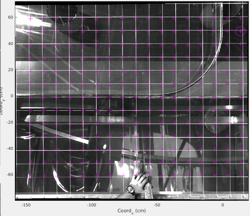
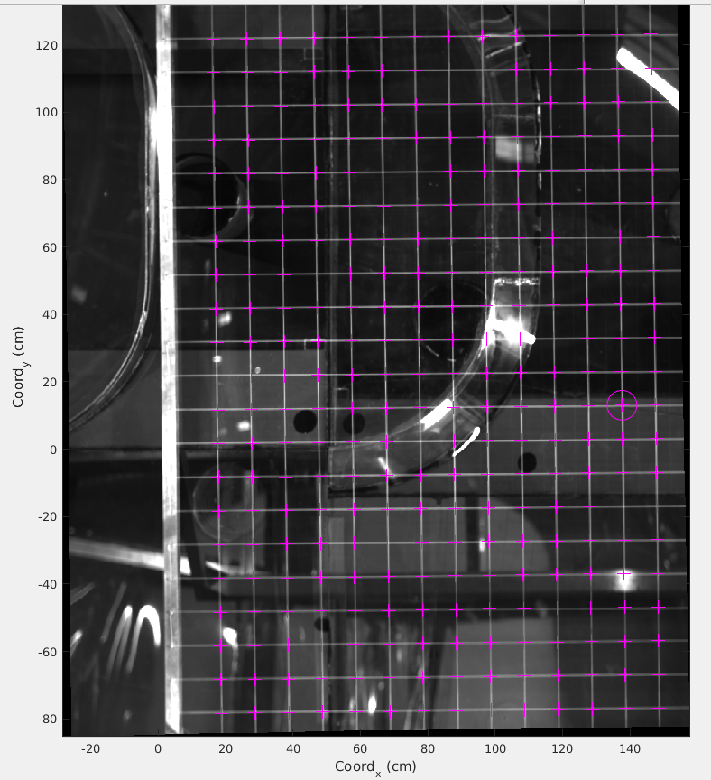
The 2D calibration is used as a reference horizontal grid with a grid height of
- z = 80.8 cm for PCO1
- z = 58.2 cm for PCO2


Calibration of camera 1 (PCO1) on the left and of camera 2 (PCO2) on the right, with the calibration grid produced with PIV in purple.
The calibration is checked with a calibration ruler (images saved in CALIB_RULER) to see that the transition between the two cameras is smooth.
For the vertical calibration the images are saved in a different file format with extension '.seq'. The format can be changed in the UVMAT software, but the folder with the vertical images should not be renamed (e.g. '2017-09-08T16.04.32'). To change the image format, choose RUN -> Field Series. Chose the right input file, an select 'extract_rdvision.m', click INPUT and RUN. The image will be saved in a new folder as a .png file and is ready for use in UVMAT.
Laser sheet calibration
| Laser setting | $H_{real} |
| 650 | 55 cm |
| 700 | 49.5 cm |
| 800 | 40 cm |
| 850 | 35 cm |
| 900 | 30 cm |
Probes calibration
For the calibration of the probes 3 measurements were done before the experiments on the 5 probes and 4 measurements were done after. For each C you can see in the table the voltage measured. Done the 21/09/2017
| $\rho$=998.9 T=20.3 | $\rho$=1004.5 T=20.7 | $\rho$=1015.1 T=21.0 | |
| C2 | -4.89 | -2.73 | 1.04 |
| C1 | -4.88 | -2.59 | 1.31 |
| ?C0 | -4.82 | -2.50? | 1.02 |
| ?C5 | -4.8? | -0.75? | X |
| C4 | -4.74 | -1.98 | 2.54 |
| T2 | X | 1.44 | 1.44 |
| T0 | X | 5.15 | 5.16 |
| T5 | X | -5.00 | X |
| T4 | X | -1.22 | 1.25 |
Done the 29/9
| $\rho$=998.2 T=22.8 | $\rho$=1004.3 T=22.3 | $\rho$=1009.5 T=22.4 | $\rho$ = 1014.9 T=22.4 | |
| C0 | -4.95 | -2.67 | -0.94 | 0.60 |
| C1 | -4.94 | -2.34 | -0.21 | 1.92 |
| C2 | -4.95 | -2.72 | -0.89 | 1.05 |
| C4 | -4.87 | -2.12 | 0.11 | 2.2 |
| C5 | -4.91 | -1.60 | Variable | X |
| T0 | 3.10 | 3.22 | 3.21 | 3.53 |
| T1 | X | X | X | X |
| T2 | X | 1.1 | 1.07 | 1.07 |
| T4 | -1.49 | -1.42 | -1.45 | -1.43 |
| T5 | -4.99 | -5.0 | -5.0 | X |
4.2 Calibration for ice shelf experiments
The images for PIV (PC01, PC02) are calibrated from images of a horizontal grid, in 3D with an inclined grid (tilted angles) and in the vertical (FALCON) for the camera fixed on the tank wall.
The calibrated images with the grids are stored in 0_REF_FILES/CALIB2 with the
- 2D calibration in the directory CALIB_09_10_horizontal
- 3D calibration in the directory CALIB_09_10_3D and CALIB_09_10_3D_2.
- calibration with the grid lying on the 2% sloping topography in the directory CALIB_09_10_2percent and CALIB_09_10_2percent_with_mark.
- Vertical calibration in the directory CALIB_27_10_vertical and CALIB_27_10_vertical_ruler.
For the calibration of PCO1 and PCO2, only the 2D calibration was used, because the 3D intrinsic parameters could be taken from the shelf break experiments.Calibration parameters are therewith stored in CALIB_09_10_horizontal.
For the calibration of FALCON, the images were too dark, so three points of the topography (bottom, upper points of the V-shape) from EXP03 were used for the calibration. The coordinate system has to be rotated keeping a right-handed CO-system, in order to apply the calibration also to the scans with the vertical laser. The axis towards Falcon has to be the z-axis (positive towards camera) to set the slices, the coordinate to the right (towards the rotating platform) is x and the upwards coordinate is y.

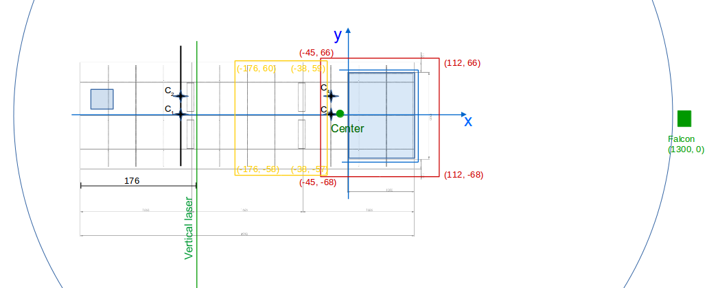
This sketch shows the topography of ice shelf together with the view of the two cameras.
The 3D calibration is done with the geometric calibration function on UVMAT to create 'intrinsic parameters' for each camera that will be used for all images. Calibration points along the inclined grid are marked and translated from image coordinates to physical coordinates defined in section 2.3.1 to later take into account the different height of slices. See http://servforge.legi.grenoble-inp.fr/projects/soft-uvmat/wiki/UvmatHelp#GeometryCalib for details of the method. The calibration parameters are copied in a xml file beside the folders of each camera (for instance PCO2.xml for PCO2/). The xml files also containing all the timing information and have to be copied next to the folders of all images, to use the same intrinsic calibration data for each image taken with the corresponding camera.
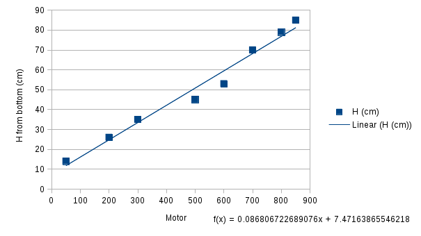
Laser sheet calibration
| Laser setting | $H_{real}$ |
| 50 | 14 cm |
| 200 | 26 cm |
| 300 | 35 cm |
| 500 | 45 cm |
| 600 | 53 cm |
| 700 | 70 cm |
| 800 | 79 cm |
| 850 | 85 cm |

Probes calibration
For the calibration of the probes 3 measurements were done before the experiments on the 5 probes and 4 measurements were done after. For each C you can see in the table the voltage measured.
First calibration: Done the 23.10.2017
| Rho_ref | T_ref | T0 | C0 | C1 | C2 | T2 | C4 | T4 |
| 998.8 | 20.4 | 1.67 | -5.02 | -4.99 | -4.95 | 1.61 | -4.83 | -1.14 |
| 999.8 | 20.0 | 2.19 | -4.51 | -4.12 | -4.06 | 1.69 | -3.60 | -1.14 |
| 1002.3 | 20.0 | 2.18 | -3.32 | -1.88 | -1.96 | 1.72 | -1.08 | -1.10 |
| 1004.5 | 21.1 | 2.39 | -2.31 | 0.18 | 0.10 | 1.47 | 1.31 | -1.23 |
Second calibration: Done the 31.10.2017
| Rho_ref | T_ref | T0 | C0 | C1 | C2 | T2 | C4 | T4 |
| 998.9 | 19.1 | 3.44 | -4.98 | -4.93 | -4.95 | 1.95 | -4.85 | -0.98 |
| 999.5 | 19.2 | 3.49 | -4.62 | -4.4 | -4.42 | 1.92 | -4.18 | -0.96 |
| 1000.2 | 19.1 | 3.51 | -4.27 | -3.84 | -3.84 | 1.98 | 3.44 | -0.94 |
| 1001.2 | 19.0 | 3.54 | -3.83 | -3.1 | -3.07 | 1.98 | -2.43 | -0.93 |
| 1002.1 | 19.1 | 3.55 | -3.45 | -2.4 | -2.33 | 1.97 | -1.5 | -0.93 |
This tables are saved on the server in 17ICESHELF/0_REF_FILES/CALIB2/Calibration_Probes_23_10.odt and Calibration_Probes_31.10.odt
5 - Good to know…
5.1 How to turn on and off the lasers

The laser for horizontal slices is turned on and off in the rotating office via the computer. You only have to switch the shutter between on and off.

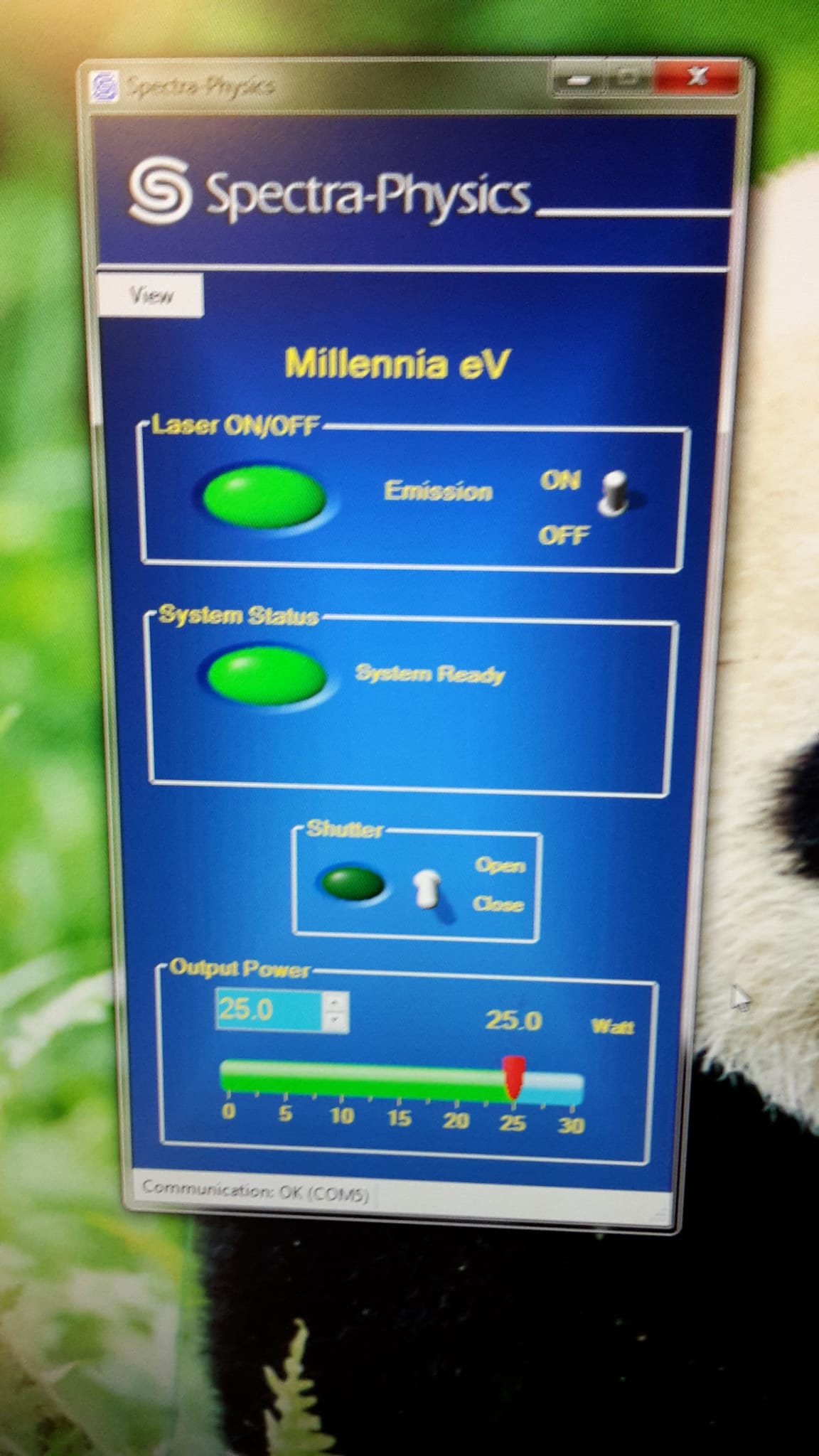
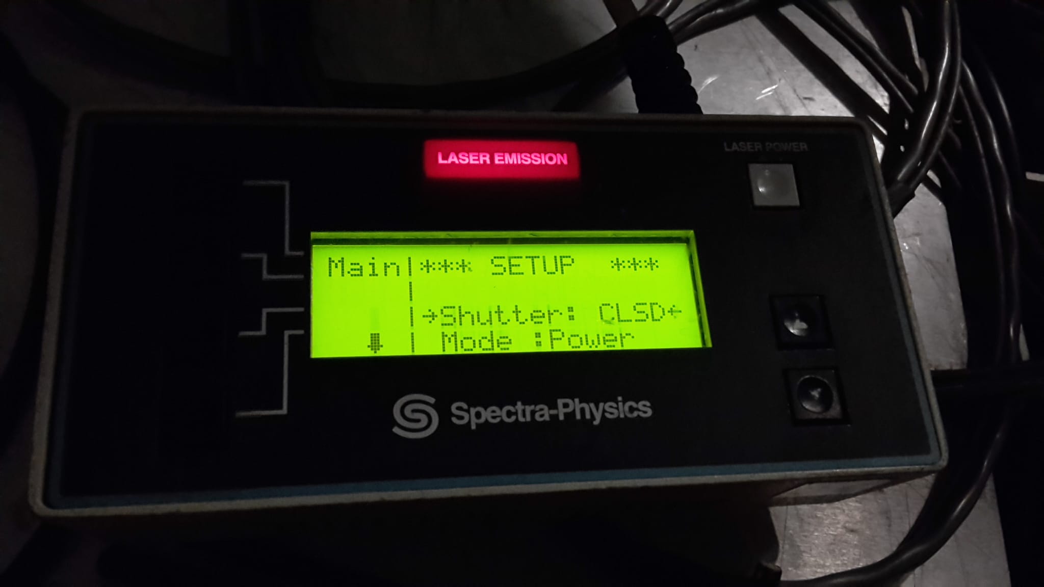
The laser for the vertical slices is turned on and off outside the wall, where the laser is located. Press the button in the lower right corner of the instrument in the photo.
5.2 How to process the data
All experiments are saved in fsnet>project>coriolis>2017>17ICESHELF>DATAZ>EXPXX. DATAZ corresponds to DATA for the slope front experiments and to DATA2 for the ice shelf experiments. The file EXPXX is for the horizontal laser sheet, EXPXX_SCAN is for the horizontal scanning and EXPXX_VERT for the vertical sheet. Within each EXPXX and EXPXX_SCAN you will get three files : FALCON, PC01 and PC02. These are the three cameras we are using during the experiments, the FALCON is the camera for the vertical sheet and will only be used to get the time parameters. The data from the PC01 and PC02 need to be treated in order to perform the PIV.
- Copy the files from the computer of the cameras.
- The images from the vertical camera are saved on the local computer in G: and have to be copied into the folder FALCON in the corresponding experiment.
- The images from PCO1 (camera at the inflow) are saved on D: of the remote desktop connection that ends with 151. The images have the be copied into the folder PCO1 of the corresponding experiment.
- The images from PCO2 (camera above the trough) are saved on D: of the remote desktop connection that ends with 150. The images have to be copied into the folder PCO2 of the corresponding experiment. - Get the .xml file with timing information
In uvmat select the Run>field series then open>browse and select an experiment. Go in the folder within the FALCON and select the .seq file. Choose extract_rdvision_times in the Action part, click on Input and Run. This will create a Falcon.xml within the FALCON folder. Check that the Falcon.xml file contains the right information on Dti (time between two images), Exposure time and Number of images (NbDti)! - Convert .tif into .png
In Run>Field series you can open any .tif of the desired folder (Warning : you should not take the im.tif but any im@… is working). Then in the Action part you should select extract_multitif, if the Input button is in pink you should click on it and give to the software the Falcon.xml that you extracted earlier (If that doesn't exist, copy one .xml file from a previous experiment and change the setting manually. Once it is done you can click on RUN, don't forget to select cluster_oar in the run mode, the action will be much faster. When it is done a new folder called PCOY.png is created in your EXPXX folder and contains all the png.
For SCANS: Check that the right number of slices is registered! To do so, click on check_data_files in the Action part and type the right number of slices in nb_slices i - Remove background
Browse for the right experiment again and chose the extracted .png images. The action sub_background that will remove all the motionless structures. For the input you have to make sure that the image rescaling coefficient is equal to 2 and then make is run. (This process takes a long time, don't forget to make it run on the cluster). You can check on Status, how many images are done. The output of this action is a file PCOY.png.sback filed with png images.
For SCANS: Here, the image rescaling coefficient should be equal to 0! Also, set the Number of images for sliding background to the number of images per slice! - Do PIV
Browse for the images with the removed background (PCOY.png.sback.). Choose the Action civ_series. For in Input, you have to import an existing .xml file to get the right parameters. You can use one .xml file from another experiment on which the piv is already done. Browse for: EXPXX/PCOY.png.sback.civ/0_XML and choose any of the img_#.xml. Make sure in the Input parameters that you chose the correct mask (right camera and with/without corner). - Add calibration grid
To get all images in cm relative to our coordinate system, the calibration we did in the beginning has to be applied on all experiments. This can be done in the very end.
Chose any experiment and any image in uvmat and chose Tools>geometry_calib>replicate. Click on NO, when ask if to apply on cropped images.Click okay on points that are off, if not too far off and click off for the assumed slice height. In the browser, chose a random file and select. In the window "browse_data", chose the data you want to apply the calibration on in the left column and chose the right Data Series on the right column (e.g. PCO1 for PCO1). The calibration will now be attached to all .xml files with the timing. - Set slices
To merge the two cameras, the slices first have to be brought to the right height. You do that by chosing any image from the right experiment. Chose Tools>Set_slices chose the height at which the laser sheet was, or the height of the first and last laser sheet and indicate the number of slices. Also important to check off refraction and type the water level. Refraction index should stay the default 1.33. For the ice shelf experiments, you can indicate the tilt of the laser layer by typing the 1.15% tilt angle y axis. The slice height can be replicated in the same way as the calibration data - Merge cameras
Important to do during PIV processing:
- Check that the Falcon.xml file contains the right information on Dti, Exposure Time and NbDti!
- Check that all files are processed before you continue!
- If there is a message about the wrong number of i before starting the civ_series, then the NbDti? in the Falcon.xml is wrong and you have to change it!
- Before pressing the RUN button always double check that it is actually analysing all images (the values in first and last in the middle section).
- If you are analysing scans and slices, always check that you have the right number of slices.
6 - Organization of data files
All data related to the project are in: \fsnet\project\coriolis\2017\17ICESHELF
- 0_DOC: miscellaneous documentation, drawings of the setup, logsheets and excel sheets with parameters
- 0_MATLAB_FCT: specific matlab functions
- 0_PHOTOS: photos of set-up, team and experiments
- 0_REF_FILES:
- CALIB1: Calibration photos and documents for Shelf Break experiments
- CALIB2: Calibration photos and documents for Ice Shelf experiments
- DATA: Raw and processed data from Shelf Break experiments
- DATA2: Raw and processed data from Ice Shelf experiments
- The DATA folders are divided into subfolders for each EXPXX with three different possibilities:
- EXPXX is for horizontal slices/ EXPXX_SCAN is for experiments in which horizontal laser scanned through layers. They contain the same subfolders:
- FALCON: The camera always run together with the PCO cameras to save the timing information in the .xml file
- PCOY: raw images for the two top-cameras (PCO1 and PCO2), that were always run synchroneously
- PCOY.png: images in .png formate
- PCOY.png.sback: .png images at which the background is removed
- PCOY.png.sback.civ: .nc files with coordinate and velocity data for Civ1 and Civ2, error information etc.
- PCO1.png.sback.civ-PCO2.png.sback.civ.mproj: .nc-files that contain coordinates, velocity, norm, curl, div, strain for the merged PCO1 and PCO2.
- PCOY.png.mask: Contains .png files of the masks.
- PCOY.xml contains the timing information for the experiment.
- EXPXX_VERT contains vertical photos taken with FALCON
- MASKS: Masks for the different experiments are saved here.
- EXPXX is for horizontal slices/ EXPXX_SCAN is for experiments in which horizontal laser scanned through layers. They contain the same subfolders:
- The DATA folders are divided into subfolders for each EXPXX with three different possibilities:
- DATA_Labview contains the data from the vertical profilers (sondes) as .lvm files.
7 - Diary for Shelf Break Experiments:
7.1 Thursday 07 September
The cameras still have to be adjusted. After that is done, we take photos with the calibration grid in the horizontal and in 3D with both cameras that are fixed on the roof. With PIV, we conduct the calibration of both cameras as described in 4.1.
7.2 Friday 08 September
To verify the calibration, we took photos with both cameras with one ruler to see if the calibrations of the cameras agree (which it does!). Then, we added a wall into the tank to prevent the water of the freshwater experiments to return to the source. The laser height was adjusted.
7.3 Monday 11 September
The table starts rotating for the first time with a velocity of 50 rounds/ sec. It gets slowly filled with water to a level of 60 cm. This takes about 3h.
After filling the tank Thoma measured the water level to be point where water level does not change with rotation 60.4 cm Center of tank – 42.5 + 16 cm = 58.5 cm Tank wall (6.5 m) – 62.4 cm. Water temperature 23.3C.
Particle sedimentation test : Water was taken from the tank, mixed with particles (30 + wetting agent) and set to settle in a glass “vase” with a narrow (ca 3cm) and tall (ca 10 cm) neck. The upper level with particles were observed as follows:
| Time | level |
| 11:50 | 0 |
| 13.05 | 4 mm |
| 13.30 | 5 mm |
At 14h40 the border was now longer visible. There were still particles in the upper part of the flask, but a lot less than there were intitally.
Calibration of vertical laser sheet
While changing the settings on the laser, the actual height of the laser sheet was measured directly in the tank.
| Laser setting | $H_{real} | |
| 650 | 55 cm | |
| 700 | 49.5 cm | |
| 800 | 40 cm | |
| 850 | 35 cm | |
| 900 | 30 cm |
We will use 650 :50: 900 to get Slices every 5 cm from 30 cm to 55 cm (total 6 Slices).
TEST experiments
The desired flow rate of 50 L/min should according to 0_DOCS\flow_rate.xclx should be achieved With a diaphragme of diameter 12.9 mm. We used 13 mm. The flow rate was estimated by measuring the time it took for the water Level in the feeding tanks to descend from 170 to 150 (with the pumps turned off) - it took 41s giving a flowrate of 40 L / 41 s = 58.5 L/min.
The pipe was first opened to remove boubles from the system. The Sources was designed in a way that the hose stopped just below the top of the Source which was out of the pater, thus creating a small waterfall, turbulence and a lot of boubles that got throught the honeycomb and flowed along the slope With the current. The Source will be redisgned so that the water is inserted below the water surface.
A second trial (still with the original source) was made later (when Samuel was back). The same ddiaphragme was used and the same amount of boubles was created. Flourescent dye (NAME) was injected first in the feeding tank above, then in directly in the water just upstream of the vertical laser sheet.
Time series of photos was obtained from the vertical camera.
Aperture 150ms Time between photos 450 ms.
There were more particles in the inflow than in the ambient, and the border between the inflow and the ambient was seen to fluctuate up and down the slope. The timescale of this motion will be estimate from the photos tomorrow.
When turning to the horizontal cameras it was decided that sloping topography gave too many uncontrolled reflections that made it unsafe to increase the intensity. To remove these,parts of the bathymetry has to be Paint in black. The tank was set to empty during the night, while recycling the water.
7.4 Tuesday 12 September
The bathymetry has been painted black, a pipe has been introduced into the source and the drain has been lowered to that it can be used also for 60 cm water depth.
The tank is filling: $T_{water}=22.9C, \rho=998.5 kg m^{-3}, T_{air} = 23C$.
The reflection is now ok and we can start our experiments!
Test experiment EXP01
We conducted experiments with a long HS from the beginning after turning on the influx (EXP_01). The influx was 41 L/min with a diaphragma of 12.6 mm diameter. The influx water had a density of 998.2 and was enriched with particles of size 30mikrom. The laser sheet was at 11cm over the trough, 4 cm over the shelf, so at 54 cm when the laser setting was at 650. We decreased it to 640 to have the laser sheet at 55 cm. Water Level (supervision - this changes witha few mm when People come enter/leave the rotating Office) was at 58.4 cm. The exposure time of the cameras was at 50ms and the time interval 500 ms.
We switched to the VS at 14:58 (EXP01_VERT).
terwards we started the Scan at 15:15 (EXP01_SCAN) with the same camera settings as for the HS. The slices were at the heights of 55 cm to 30 cm in 5 cm steps. We took 4 images at each height with a time interval of 500 ms.
Observations: On the horizontal scans we can clearly see turbulent/vertical motion along the coast. They turn left at the curvature and follow along the topography to the wall. Some particles turn right above the trough/ shelf and flow out to the slope again.
Data check: We checked these first results with the PIV and decided to decrease the exposure time to get sharper images of the particles. With PCO2, the flow around the curvature can be captured with the PIV, but on PCO1 the PIV is not very good, because the flow is more turbulent and more 3 dimensional. We decide to decrease the time between the photos. Later we realized that the cameras only took every second photo, so with a time interval of 1000ms - > useless PIV.
Experiment EXP02
We repeated the HS with a reduced time to 200 ms between the photos and and exposure time of 30ms. We realized afterwards that the cameras only took every second photo, so with a time interval of 400ms!
7.5 Wednesday 13 September
The cameras are fixed now and taking every photo and the particles are spread out in the ambient water.
Experiment EXP03
The setup is still the same as for the previous experiments with 200ms time difference between the photos (this time working!) and particles in the ambient water. This time, we measured the flow rater AFTER the experiment and it was $Q = 50 l/min$ (measurements repeated twice), as expected. There are still bubbles coming out of the source!
The current reached the first corner after about 1 minute, and the trough corner after about 3 minutes.
Experiment EXP04
We started a new experiment at !10:31 with a reduced flow rate of about $Q = 20 l/min$ (diaphrama diameter of 6.8 mm). The first HS is run for 15 min n(!10:31- !10:46). The flow field was still evolving so we extended the five more minutes of hs (!10:51-10:56 this data are stored in EXP04_B) before we started the scan ( !10:59).
Note: During the scan, the laser is shaking too much! This needs to be changed.
Observations: The bubble at the source disappeared due to the lower flow rate. The current follows along the slope and turns left at the 2nd curvature into the trough. After the 15 min after the flow was turned on, the flow bifurcates at the continental coast and at the trough and fills up the trough. The return flow does not follow along the upstream slope of the trough, but occurs in the middle of the trough. The main current along the slope is getting wider with time.
Experiment EXP05
The vertical velocity of the laser was decreased and the timestep between the first and the second image at each level increased to 1s (first image will be discarded).
The tank from where the inflow is pumped was mistakenly filled with too much Cold water (T=19.2C) - i.e. about 4 c colder than the water in the tank.
There where a lot of Bubbles coming out from the Source - and we observed large (10 cm) airbubbles travelling Down the hose during the Experiment.
All the water turned at the first water, onto the shelf.
The current was at the first corner about 1 minute after the valve was opened.
Experiment EXP06
The squared cornes were inserted - the land corner was fastened with tape and the submerged corner with a screw..
To reduce to amount of Bubbles coming out from the Source we added a thin sheet of foam behind the honey comb. In addition, the joints of the tube where the diaphragm is inserted was greased. This appeared to help - the amound of Bubbles was greatly reduced and no Bubbles was seen travelling Down the hose.
The flow separated at the first corner and turned at the second corner.
The vertical scann was started 15 min after the valve was opened.'
Experiment EXP07
An eddy initially forms behind the first corner, but it then disappears.
The flow turns into the through. Large eddy on the Continental shelf (as in Kjerstis model Experiments!).
When scanning dt was set to 100 ms, but only every second photo was aquired so dt= 2 x 100.
7.6 Thursday 14 September
Experiment EXP08
The squared corners are still on, for the first 3 minutes of the horizontal slice the light in the entrance was turned on.
The flow turned left at the second corner following the slope in the depression keeping a "tight" shape on the topography.
After a while, a straight flow established, following the slope. The circulation is very slow compared to yesterday.
For the scan there is dt =1000ms between the first and the second image at each level, then dt=400ms. First image is not used to PIV
This is to avoid shaking of laser.
Experiment EXP09
The squared corners are removed and the flow rate is reduced. There were a lot of particles in the inflow in the beginning.
There is a clear split of the flow at the 2nd corner, the main part crosses the depression following the slope and a much smaller part followed the topography inside the depression.
The laser sheets were started 26 minutes after the valve was opened.
Experiment EXP10
The flow rate is increased, there are again a lot of bubbles.
Time to reach the first corner: less than 1minute.
After the reaching the first corner a major part of the flow followed the boundary and circulated on the shelf.
A smaller part continued to the corner of the slope and the depression (after 3minutes) and entered the depression, circulated along the topography and escaped by the western side of the depression
Experiment EXP11
The water level is increased by 10 centimeters to 68.5 cm. With the higher water level, we need to calculate new flow rates with the ration of the outflow area before and after the higher water level. Now, we are aiming to a flow rate of 33 l/min, which corresponds to the 20 l/min for the lower water level.
Conversion of flow rate from low to high water level:
| Q (low water level) | Q (high water level) |
| 10 | 17 |
| 20 | 33 |
| 35 | 58 |
| 50 | 83 |
| 80 | 133 |
Note: In the previous experiment, the measured flow rate was always higher than the expected one with their diaphragme - flowrate curve. We plotted the diaphrame vs. flowrate again with the values from our experiments. For the flowrate of Q = 33 l/min, we therefore used a diaphragme with diameter of 10 mm, instead of 8.6 mm (which it was for the 20 l/min flux before).
We measured the flux 4 times during this experiment. It gave:
- 32.4 l/min
- 34.5 l/min
- 33.3 l/min
- 34.9 l/min
Measured water level after the experiment: 72.7cm at the edge and 68.5cm over the topography.
Time to reach the first corner: 3 min.
Observations: There are no more bubbles. The flow crossed the shelfbreak between the 1st and the 2nd corner. After the flow is established it follows along the rough topography and returns along the continental coast.
There was no straight flow along the slope.
There were very few particles in the end of the horizontal slice. On the vertical slice the flow does not look barotropic.
Note: After Exp11 they realized that there was water in the laser, they had to go and move it up.
Experiment EXP12
This experiment was the same as EXP11 with a water level of 68.5 cm but with the corner. The expected flowrate was 33 l/min and the measured flowrate was 34.6 l/min.
The exposure time was increased to 40 ms, because the flow is slow - so no need to have a short exposure time. It makes the particles more visible.
7.7 Friday 15 September
Experiment EXP13
During night, we increased the rotation rate to get a rotation period of 30s! We kept the corners.
There were still many particles in the ambient water, but Thomas sprayed more particles on the surface.
New measured water levels:
- wall: 69.8 cm
- center: 59.5 cm
- invariant: 65 cm
Water level on the screen: 63.4 cm
For the desired fluxrate of 50 l/min, we used the diaphragme with 12.6 mm diameter. The measured fluxrate after the experiment was 54.5 l/min.
Observations: In the beginning of the experiment, there were too many particles in the influx, but got less with time. The main current turned left at the second corner into the trough.
Note: The source is leaking, which created bubbles and a little "waterfall" due the the water surface difference inside and outside the source. Thomas fixed it by putting a wooden block in front of the leakage.
Experiment EXP14
We increase the influx to a desired value of 80 l/min with still the higher water level and increased rotation rate. Due to the leak there are water bubbles at the surface of the water at certain places.
Due to the high flux rate, we use an exposure time of 30 ms and a dt of 100ms.
Notes: The water level increased constantly. After this experiment, we had to adjust the sink to let out more water. It takes some time, so we had to wait until the water level was good again.
Water level on the screen : 63.4cm. The desired flux rate was 80L/min, we used the 16mm diaphragm and measured a rate of 94.7L/min.
Observations : The flow took 20s to reach the first corner, nothing crosses the shelf, a circulation is created on the shelf by water turning on the 1st or 2nd corner.
After a while some part of the current started following the slope after the 2nd corner.
Experiment EXP15
We wait for the water level to decrease (for about 2 hours) and reach 62.7cm on screen.
The desired flow rate is 50L/min and with the diaphragm of 12.6mm we measured a flow rate of 52.2L/min.
Observations : The flow reaches the first corner very quickly, then turned to the left and circulated on the shelf quite fast. Then a second branch started circulating inside the depression following the bathymetry.
After that a third smaller branch started to follow the slope.
Note : After this experiment, inertial oscillations appeared and the water started to move so we had to wait until further experiments.
Experiment EXP16
When we started this experiment the inertial oscillations were reduced but not suppressed.
The desired flow was 35L/min, with the diaphragm of 10mm we measured 36L/min.
Observations : At the first corner a large part of the flow turned left and went on the shelf, circulating in a larger vein than the previous experiment.
Some water reaches the 2nd corner splitting in a major part entering the depression and a smaller and slower part flowing along the slope.
There was no recirculation inside the depression, all the flow was evacuated at the end of the depression bypassing the "land".
Experiment EXP17
At the beginning of the experiment there were almost no oscillations left.
The desired flow was 20L/min, with a diaphragm of 8.2mm we measured 21.6 L/min.
Observations : At the 1st corner the flow continued straight ahead. At the 2nd corner the flow split in 2 branches of equal size, one following the slope and on entering the depression.
There was a very clear and narrow jet following the bathymetry inside the depression, with a lot of meanders on its sides.
After a while a branch detached from the slope current at the western corner of the depression entered the depression and recirculated joining the eastern side of the depression (drawing on the experiment paper).
We wanted to keep the same setup and to increase the flow rate to 80L/min in order to have consistency but unfortunately we were running out of time.
7.8 Monday 18 September
The whole day was used to build the extension of the topography to move the source 2m further back. The source sits now at the same position relative to the topography, only 2m further back. The cameras stayed at the same positions. We used this day to process data and to learn more about UVMAT.
7.9. Tuesday 19 September
Experiment EXP18
Today, first the source had to be attached and the water filled up. Then the particles had to be spread out in the water again. So the experiment didn't start before 11:30.
At least, the source was now moved 2m further back and the foam of the source was improved to avoid bubbles leaving the source, which also worked with this flow rate.
Because the source was mainly too close for the high flow rates, we will only do experiments with flow rates higher than 50 and with a rotation rate of 50. We started with Q = 50l/min and no corner.
Observations: The flow was much more established, when it reached the view of PCO1. Regular waves occurred along the slope until it reached the first corner. Almost the whole current turned south into the trough.
Notes: The images for HS were accidentally only taken for 7min, but restarted again for 7 min (EXP18_B).
Experiment EXP19
We used the same setup at EXP18, just with a flow rate of Q=80l/min. Note that we still used the diaphragme of the original diameter-flow rate curve, which gives an actual flow rate of >90 l/min. We do that to be consistent with previous experiments.
From the PIV of previous experiments with a flow rate of 80, we have decided to decrease the dt from 100 to 50ms and also the exposure time from 30 to 20ms, because the correlations were not very high. However, the dt = 50 ms did not work during this experiment, so that in fact it was dt = 100ms, because only every second image was taken.
During this experiment, the honeycomb fell out of the source after the HS. We did therefore no vertical scan.
Note: This experiment had too many errors that we had to redo it!
Experiment EXP20
We redid experiment 19 and this time everything worked. dt is now 50ms and the exposure time 20ms. We had no corner. The measured flow rate was 93.5 l/min.
Observations: Most of the current is entering the trough and a small part passes the trough, following the slope.
Experiment EXP21
For this experiment, we wanted to increase the flow rate to Q = 110 l/min, with a diaphragme of 17 mm. The measured flow rate was 120 l/min. The experiment was again without corner and dt = 50 ms, E = 20 ms.
Observation: The whole current went into the trough.
Experiment EXP22
This experiment had the same setup as EXP21 but with the corner. The measured flow rate this time was only 100 l/min.
Note: The flow rate is difficult to measure for high values, as the time interval is shorter and therefore produces a larger error. However, in the end we can plot a diameter - flow rate curve fitted with all the values from our experiment. The diaphragme should determine the flow rate quite clearly and with the fitted curve, we can get the actual flow rate.
Observations: Most of the current went into the trough, only a small part passed by. There were many particles in the beginning of the experiment.
7.10 Wednesday 20 September
Experiment EXP23
After swirling up the particles in the tank, we started early at 08:13 with the first experiment. It is the same experiment as EXP22 with a flow rate of Q=80l/min. The calculated flow rate is 94 l/min, which is very close to the previous flow rate (100l/min).
Observation: The flow was similar to the previous experiment, with the main current entering the trough. A large rotation occurred on the shelf.
Experiment EXP24
We increased the water level to 70 cm and kept the corner. The plan was to do one experiment with Q=110 l/min, but because that was so similar to 80 l/min before, we decided to increase it to 150 l/min (diaphragme 19.5mm). Measurements of the flow rate gave a value of Q = 150 l/min. We kept the small dt = 50 ms and the E = 20 ms.
Observations: The current entered the trough in a very large radius and builds an anti-cyclone on the shelf. Only a very small part of the current went straight, passing the trough.
Note: During this and the following experiments with a water level of 70 cm, we didn't convert the flow rate relative to the source area below the water level! So, all these experiments give a smaller velocity compared to the same experiments with the lower water level.
Experiment EXP25
The desired flow rate was reduced to 80 l/min (diaphragme 16mm), which gave a flow rate of 94 l/min.
Observations: At the slope current towards the first corner, large vortices were created. The inflow into the trough was not very strong and more turbulent. Half of the flow passed the trough along the slope.
Experiment EXP26
The desired flow rate was reduced to 50 l/min (diaphrame 12.6mm), which gave a flow rate of 54 l/m. The images were started after the flow started, because it takes a long time for the flow to reach the view of the first camera.
Note: The images for the first HS were taken for too short time (10 min), so that the flow was not established yet. We restarted and took more images for 5 min (saved in EXP26_B).
Note: We added larger particles (60 micron) into the inflow water (instead of the 30 micron), because Joel suggested that it may be better for the PIV. The particles in the ambient water were still the same.
Observations: The current enters the trough in a very large radius.
Experiment EXP27
This is a repetition of EXP26 without the corner. The measured flow rate was 53.2 l/min.
Observations: Compared to EXP26 with the corner, the current enters the trough in a much smaller radius, following neatly the topography. After waiting, also a large part flow straight.
Note: In the beginning of the experiment, there were still a lot of particles in the ambient water.
Experiment EXP28
The desired flow rate was increased to 80 l/min (16mm), which gave a measured flow rate of 92.4 l/min.
We had to do this experiment twice (first one was overwritten), because the honeycomb in the source loosened in the beginning of the first time and released a lot of clustered particles/bubbles that spread over the whole flow area. The source had to be fixed and we didn't have the time to completely wait until all the clusters escaped the tank. During the second round of this experiment, there were therefore still some of the clusters moving into the sight of the cameras.
Observations: The largest part of the current continued straight, but there was quite a strong return flow across the trough from the western corner of the trough to the southeastern corner of the trough.
7.11 Thursday 21 September
During the night, the tank was emptied. This day was used to fix the 5 probes for the vertical salinity profiles, they were set up and tested. The lower part of the source was covered with tape to only get a squared inflow. Then, the tank was filled up with salt water (density of 11.0 kg/m3) and turned into solid body rotation with T=50s.
7.12 Friday 22 September
Today, the baroclinic experiments started. The density of the inflow was 1.2 kg/m3 to get a density difference of 9.8 km/m3. We were told that it is easier to increase reduce the density difference by adding salt in the inflow than to decrease it (However, after all we can switch between the two quite easily). Due to the higher density, we used 60 micron particles in the ambient and the inflow water.
Experiment EXP29
During this experiment, we started with a HS (20 min), run the profiles with the probes as soon as the inflow was established (while doing the HS) and did the vertical slice (2 min) and the scan afterwards.
The flow rate of 20 l/min (8.5mm diameter) gave a measured flow rate of 20 l/min.
Probes: downward velocity: 2 cm/s; upward velocity: 5 cm/s; break at the surface: 10s. In total 10 repetitions. The height of the probes are adjusted to follow the slope. They start about 20.5 cm above the slope so that only the probe furthest away from the coast touches the water, the others stay above the surface. During the profiles they get lowered by 19 cm.
Scans: 11 levels (55:-2:35) with 5 images at each level. dt = 100ms and dt1 = 1000ms. Exposure time was 30ms.
Observations: The flow was very fast and a nice clear front developed. In the beginning the water formed a vortex just after the first corner, and then most of the flow entered on the shelf between the first and the second corner. On the vertical slice, the front was clearly visible, but it was very steep, so that it may be above the laser sheets.
Note1: The vertical camera is too far up for the experiments with density difference, as the free surface is not visible. It will be put further down for the following experiments.
Note2: The second probe from the coast is not working properly!!
Note3: We have to remember that the source area is smaller and the flow therefore higher!
Experiment EXP30
The flow rate was increased to 50 l/min (12.6mm diameter), which gave a measured flow rate of 53 l/min. The flow was very high and the dt therefore reduced to 50ms and Exposure time was reduced to 20ms after a few minutes (saved in Exp_B).
Probes: We kept the same setup as EXP29, but did now 20 profiles.
Observations: The flow turn onto the shelf at the second corner and followed the topography also on southern side of the topography. After a while, a vortex developed in the trough and parts of the main flow entered this vortex.
Note: In the beginning of the experiment, the water was still in motion from the previous experiment due to the density difference.
Experiment EXP31
The flow rate was increased even more to 80 l/min (14mm diameter), which gave a measured flow rate of 75 l/min. As in the previous experiment, the we always got too high flowrates for the 80 l/min - experiments with the 16mm diameter, we decided to now chose a smaller diameter. We were also concerned that it was not possible to do PIV with an ever faster flow, because it is not possible to use a dt < 50 ms and E<20!
Observations: All water turned onto the shelf at the 2nd corner and formed a vortex over the shelf. Some of the flow turned within the trough in a very wavy way (didn't follow the topography out of the trough again).
Experiment EXP32
Now, we removed the corner and did an experiment with 50 l/min flow rate (12.6 mm), which gave 52 l/min. dt = 50ms, E=20ms.
Observations: The flow went straight around the 1st corner and followed the topography.
Notes: The water was still in motion in the trough from the previous experiment and due to the density difference. It looked like the particles started settling down, which may create vertical motion. It may be, that there was already a fresh water layer at the surface that influenced the flow, but also the laser height.
Experiment EXP33
This experiment was with a low flow rate of 20 l/min and had to be stopped after a while as there was a too strong stratification. The laser then got deflected downward at the interface between the two densities and was only about 1-0 cm above the topography on the shelf.
7.13 Monday 25 September
Experiment EXP34
We did NOT redo experiment EXP33! Instead, we increased the inflow density to get a difference of about 5 kg/m3 (measured: 4.8 kg/m3). The measured water level was 58.4 cm in the centre and the laser sheet was at 55 cm in the centre. We started with an inflow of 20 l/min (8.5mm) which measured 22.3 l/min.
Experiment EXP35
The inflow was increased to 50 l/min.
Note: At the beginning of the experiment, the water was not completely at steady-state in the trough. The scans were supposed to do 550 images, but only took 500. And it only did 10 levels, instead of 11, so the last level is missing!
8 - Table with Shelf Break experiments
- A complete list of all experiments with comments is saved in LIST_OF_EXPERIMENTS.xlsx
| Exp No. | Name | Valve opened | $H_{water}$ | $T_{rot}$ | $Q$ | $R_{curvature}$ | $\Delta \rho$ | Diaphragme | Flowrate estimated | Type of photo | Height of HS | Heights of Scan and # | Time photo | Dye | Comments | Notes |
| $(m)$ | $(s)$ | $(L min^{-1})$ | $(m)$ | $(kg m^{-3}$ | $(mm)$ | $H_1,H_2,\Delta t $ | VS/HS/Scan | $cm$ | $cm$ | t1/t2/t3 $\Delta t$ | yes / no | |||||
| 0 | test | 11092017 hh:mm | 0.604 | 50 | 58.5 | 0.50 | 0 | 13 | 170,150,41s | VS | - | - | ? | yes | Dye did not show up in photos :-( | Elin |
| 1 | exp01 | 12092017 !14:38 | 0.584 | 50 | 40.67 | 0.50 | 0 | 12.6 | 170,150,59s | HS,VS,Scan | 55 | 55:[-5:30,4 -5:30;4] | 500ms (reality: 1000ms) | no | Expl. time = 50 ms too little. Only every second photo was taken | Elin |
| 2 | exp02 | 12092017 !17:02 | 0.583 | 50 | 44.2 | 0.50 | 0 | 12.6 | 180,150,81.4s | HS | 55? | - | 200ms (reality: 400ms) | no | Only every second photo was taken | Elin |
| 3 | exp03 | 13092017 | 50 | 50 | 0.50 | 0 | 12.6 | HS,Scan | 200ms | no | Problem with photos fixed; particles in ambient | Elin | ||||
| 4 | exp04 | 13092017 | 50 | 0.50 | 0 | 6.8 | HS,Scan | 200ms | no | Laser started vibrating for the scans | Elin | |||||
| EXP | Date | T (s) | Q (l/min) | Corner | dRho (kg/m³) |
| 1 | 20170912 !14:38 | 50 | 50 | no | 0 |
| 2 | 20170912 !17:02 | 50 | 50 | no | 0 |
| 3 | 20170913 !08:53 | 50 | 50 | no | 0 |
| 4 | 20170913 !10:31 | 50 | 20 | no | 0 |
| 5 | 20170913 !14:02 | 50 | 80 | no | 0 |
| 6 | 20170913 !17:55 | 50 | 80 | yes | 0 |
| 7 | 20170913 !17:55 | 50 | 50 | yes | 0 |
| 8 | 20170914 !09:23 | 50 | 20 | yes | 0 |
| 9 | 20170914 !10:38 | 50 | 10 | no | 0 |
| 10 | 20170914 !11:35 | 50 | 35 | no | 0 |
| 11 | 20170914 !14:27 | 50 | 33 | no | 0 |
| 12 | 20170914 !17:15 | 50 | 33 | yes | 0 |
| 13 | 20170915 !09:16 | 30 | 50 | yes | 0 |
| 14 | 20170915 !10:33 | 30 | 80 | yes | 0 |
| 15 | 20170915 !13:12 | 30 | 50 | no | 0 |
| 16 | 20170915 !15:11 | 30 | 35 | no | 0 |
| 17 | 20170915 !16:02 | 30 | 20 | no | 0 |
| 18 | 20170919 !11:31 | 50 | 50 | no | 0 |
| 19 | 20170919 !14:13 | 50 | 80 | no | 0 |
| 20 | 20170919 !15:08 | 50 | 80 | no | 0 |
| 21 | 20170919 !15:47 | 50 | 110 | no | 0 |
| 22 | 20170919 !16:45 | 50 | 110 | yes | 0 |
| 23 | 20170920 !08:13 | 50 | 80 | yes | 0 |
| 24 | 20170920 !10:08 | 50 | 150 | yes | 0 |
| 25 | 20170920 !11:12 | 50 | 80 | yes | 0 |
| 26 | 20170920 !14:01 | 50 | 50 | yes | 0 |
| 27 | 20170920 !14:40 | 50 | 50 | no | 0 |
| 28 | 20170920 !16:14 | 50 | 80 | no | 0 |
| 29 | 20170922 !09:43 | 50 | 20 | yes | 10 |
| 30 | 20170922 !11:06 | 50 | 50 | yes | 10 |
| 31 | 20170922 !14:30 | 50 | 80 | yes | 10 |
| 32 | 20170922 !15:16 | 50 | 50 | no | 10 |
| 33 | 20170922 !16:05 | 50 | 20 | no | 0 |
| 34 | 20170925 !09:34 | 50 | 20 | no | 5 |
| 35 | 20170925 !10:30 | 50 | 50 | mo | 5 |
| 36 | 20170925 !11:38 | 50 | 80 | no | 5 |
| 37 | 20170925 !14:51 | 50 | 20 | yes | 5 |
| 38 | 20170925 !15:11 | 50 | 80 | yes | 5 |
| 39 | 20170925 !16:53 | 50 | 110 | yes | 5 |
| 40 | 20170926 !9:38 | 30 | 20 | no | 5 |
| 41 | 20170926 !10:22 | 30 | 50 | no | 5 |
| 42 | 20170926 !11:37 | 30 | 10 | no | 5 |
| 43 | 20170926 !14:22 | 30 | 5 | no | 5 |
| 44 | 20170926 !15:32 | 30 | 5 | no | 5 |
| 45 | 20170926 !16:43 | 30 | 20 | yes | 5 |
| 46 | 20170927 !9:00 | 30 | 5 | yes | 5 |
| 47 | 20170927 !10:32 | 30 | 50 | yes | 5 |
| 48 | 20170927 !14:01 | 30 | 5 | no | 3 |
| 49 | 20170927 !14:47 | 30 | 20 | no | 3 |
| 50 | 20170927 !16:05 | 30 | 50 | no | 3 |
| 51 | 20170928 !09:30 | 30 | 5 | yes | 3 |
| 52 | 20170928 !10:45 | 30 | 20 | no | 3 |
9 - Table with Ice Shelf Experiments
More details and comments on all experiments are attached in EXPERIMENTS_ICESHELF_WikiPage.xlsx
| EXP | Date | T (s) | dH (cm) | Q (l/min) | dRho (kg/m³) | |
| 1 | 09/10/17 16:57 | 60 | 0 | 50 | 0 | |
| 2 | 10/10/17 10:20 | 60 | 0 | 30 | 0 | |
| 3 | 10/10/17 14:03 | 60 | 5 | 30 | 0 | |
| 4 | 10/10/17 14:59 | 60 | 10 | 30 | 0 | |
| 5 | 10/10/17 15:49 | 60 | 15 | 30 | 0 | |
| 6 | 10/10/17 16:36 | 60 | 15 | 50 | 0 | |
| 7 | 11/10/17 10:11 | 60 | 20 | 30 | 0 | |
| 8 | 11/10/17 10:11 | 60 | 20 | 30 | 0 | |
| 9 | 11/10/17 13:47 | 60 | 0 | 30 | 0 | |
| 10 | 11/10/17 15:35 | 60 | 0 | 30 | 0 | |
| 11 | 11/10/17 16:38 | 60 | 0 | 15 | 0 | |
| 12 | 12/10/17 08:35 | 60 | 15 | 30 | 0 | |
| 13 | 12/10/17 10:23 | 60 | 30 | 30 | 0,4 | |
| 14 | 13/10/17 08:15 | 30 | 30 | 30 | 0 | |
| 15 | 16/10/17 09:22 | 30 | 0 | 30 | 0 | |
| 16 | 16/10/17 11:16 | 30 | 0 | 30 | 0 | |
| 17 | 16/10/17 14:25 | 30 | 0 | 50 | 0 | |
| 18 | 16/10/17 15:39 | 30 | 15 | 50 | 0 | |
| 19 | 16/10/17 16:29 | 30 | 15 | 30 | 0 | |
| 20 | 17/10/17 08:35 | 30 | 30 | 50 | 0 | |
| 21 | 17/10/17 08:40 | 30 | 30 - 0 (tilted) | 50 | 0 | |
| 22 | 17/10/17 11:12 | 30 | 30 - 0 (tilted) | 30 | 0 | |
| 23 | 17/10/17 14:30 | 30 | 30 - 15 (tilted) | 30 | 0 | |
| 24 | 17/10/17 15:51 | 30 | 30 - 15 (tilted) | 50 | 0 | |
| 25 | 19/10/17 09:20 | 30 | 30 | 50 | 0 | |
| BUILT WALL: | ||||||
| 26 | 19/10/17 13:46 | 30 | 30 | 50 | 0 | |
| 27 | 19/10/17 14:47 | 30 | 30 | 30 | 0 | |
| 28 | 19/10/17 16:02 | 30 | 30 | 30 | 1 | |
| 29 | 20/10/17 09:19 | 30 | 30 - 0 (tilted) | 30 | 0 | |
| 30 | 20/10/17 10:39 | 30 | 30 - 0 (tilted) | 60 | 0 | |
| 31 | 20/10/17 13:42 | 30 | 30-15 (tilted) | 60 | 0 | |
| 32 | 20/10/17 14:44 | 30 | 30 - 15 (tilted) | 30 | 0 | |
| 33 | 20/10/17 16:34 | 30 | 0 | 30 | 0 | |
| 34 | 23/10/17 08:41 | 30 | 0 | 60 | 0 | |
| SOURCE MOVED DOWNSTREAM | ||||||
| 35 | 23/10/17 09:44 | 30 | 0 | 60 | 0 | |
| PROBES PUT IN PLACE | ||||||
| 36 | 23/10/17 16:07 | 30 | 0 | 60 | 1 | |
| 37 | 23/10/17 16:58 | 30 | 0 | 30 | 1 | |
| 38 | 24/10/17 08:50 | 30 | 30 | 30 | 1 | |
| 39 | 24/10/17 09:45 | 30 | 30 | 60 | 1 | |
| 40 | 24/10/17 10:40 | 30 | 30-15 (tilted) | 60 | 1 | |
| 41 | 24/10/17 11:21 | 30 | 30-15 (tilted) | 30 | 1 | |
| 42 | 24/10/17 13:45 | 30 | 30-15 (tilted) | 30 | 2 | |
| 43 | 24/10/17 14:35 | 30 | 30-15 (tilted) | 60 | 2 | |
| 44 | 24/10/17 15:22 | 30 | 30-0 (tilted) | 60 | 2 | |
| 45 | 24/10/17 16:04 | 30 | 30-0 (tilted) | 30 | 2 | |
| 46 | 24/10/17 16:42 | 30 | 30-0 (tilted) | 30 | 2 | |
| 47 | 25/10/17 08:36 | 30 | 30-0 (tilted) | 60 | 1 | |
| 48 | 25/10/17 09:09 | 30 | 30-0 (tilted) | 30 | 1 | |
| 49 | 25/10/17 10:20 | 30 | 30 | 30 | 2 | |
| 50 | 25/10/17 10:58 | 30 | 30 | 60 | 2 | |
| 51 | 25/10/17 13:59 | 30 | 0 | 60 | 2 | |
| 52 | 25/10/17 15:19 | 30 | 0 | 30 | 2 | |
| 53 | 25/10/17 15:58 | 30 | 0 | 30 | 2 | |
| 54 | 25/10/17 16:58 | 30 | 30 | 30 | 2 | |
| 55 | 26/10/17 09:26 | 30 | 30-15 (tilted) | 30 | 2 | |
| 56 | 26/10/17 10:12 | 30 | 30-0 (tilted) | 30 | 2 | |
| 57 | 26/10/17 14:19 | 30 | 30-0 (tilted) | 60 | 0 | |
| 58 | 26/10/17 15:24 | 30 | 30-0 (tilted) | 60 | 0 | |
| 59 | 26/10/17 16:40 | 30 | 30-15 (tilted) | 60 | 0 | |
| 60 | 27/10/17 09:16 | 30 | 15 | 60 | 0 | |
| 61 | 27/10/17 10:56 | 30 | 15 | 30 | 0 | |
| 62 | 27/10/17 14:34 | 30 | 0 | 30 | ||
| 63 | 27/10/17 around 16 | 30 | 0 | 30 | ||
| 64 | 30/10/17 14:05 | 30 | 0 | 30 | 2 | |
| 65 | 30/10/17 14:58 | 30 | 0 | 30 | 2 | |
| 66 | 30/10/17 15:47 | 30 | 0 | 60 | 2 | |
| 67 | 30/10/17 16:37 | 30 | 30 | 30 | ||
| 68 | 30/10/17 17:10 | 30 | 30 | 15 | ||
| 69 | 31/10/17 09:05 | 30 | 30 | 15 | 2 | |
| 70 | 31/10/17 09:44 | 30 | 30 | 30 | 2 | |
| 71 | 31/10/17 10:36 | 30 | 30 | 30 | 2 | |
Attachments (18)
- DSC_0811_00001.jpg (59.5 KB) - added by 9 years ago.
- PCO1_Calibration2.png (437.0 KB) - added by 9 years ago.
- PCO2_Calibration.png (368.8 KB) - added by 9 years ago.
-
Bathymetry_with_PositionCameras.pdf (47.4 KB) - added by 9 years ago.
Topography with the positions of the cameras
-
Bathymetry_with_Positions.pdf (56.7 KB) - added by 9 years ago.
Topography position relative to the tank walls with source
- Topography_with_PositionCameras.png (57.9 KB) - added by 9 years ago.
- Bathymetry_with_Positions.png (107.4 KB) - added by 9 years ago.
- Bathymetry_Vertical.png (25.3 KB) - added by 9 years ago.
- Bathymetry_Vertical.2.png (25.3 KB) - added by 9 years ago.
- Bathymetry_Vertical.3.png (25.3 KB) - added by 9 years ago.
- Bathymetry_Vertical.4.png (10.0 KB) - added by 9 years ago.
- horizontallaser_switch.jpg (193.0 KB) - added by 9 years ago.
- verticallaser_switch.jpg (96.2 KB) - added by 9 years ago.
- Bathymetry_with_PositionCameras.png (118.9 KB) - added by 9 years ago.
- Conversion_MotorLevel_LaserSheet.png (15.5 KB) - added by 8 years ago.
- Channel_Sideview_with_Coordinates.png (57.7 KB) - added by 8 years ago.
- Channel_with_Coordinates.png (60.8 KB) - added by 8 years ago.
- Channel_with_CameraPositions.png (42.7 KB) - added by 8 years ago.
Download all attachments as: .zip