| Version 45 (modified by , 9 years ago) (diff) |
|---|
- ICESHELF
- 0 - Publications, reports from the project
- 1 - Objectives
-
2 - Experimental setup:
- 2.1 General description
- 2.2 Topography
- 2.3 Reference axis
- 2.3.2 Reference axis for ice front experiments
- 2.4 References axis along the wall (horizontal and vertical) - Nadine …
- 2.5 Fixed Parameters
- 2.5 Variable Parameters
- 2.6 Additional Parameters
- 2.7 Definition of the relevant non-dimensional numbers (UPDATE WITH …
- 3 - Instrumentation and data acquisition
- 4 - Methods of calibration and data Processing (NADINE)
- 5 - Good to know…
- 6 - Organization of data files
- 7 - Diary:
ICESHELF
| Infrastructure | CNRS_Coriolis Topographic Barriers and warm Ocean currents controlling Antarctic ice shelf melt |
| Project (long title) | Topographic Barriers and warm Ocean currents controlling Antarctic ice shelf melt |
| Campaign Title (name data folder) | 17ICESHELF |
| Lead Author | Elin Darelius (part I) and Anna Wåhlin (part II) |
| Contributors | Nadine Steiger, Lucie Vignes, Joel Sommeria, Samuel Viboud |
| Date Campaign Start | 04/09/2017 |
| Date Campaign End | 27/10/2017 |
0 - Publications, reports from the project
1 - Objectives
The warm water threatening to melt the Antarctic ice shelves originates from the deep ocean north of the continental shelf. In order for the warm water to reach the ice shelf cavities it has to pass to topographic barriers: the shelf break and the ice shelf front. In a series of experiments we will explore the role of topography in controlling the onshelf flow of warm water.
2 - Experimental setup:
2.1 General description
The two Barriers - the shelf break and the ice shelf front - will be studied in two separate sets of Experiments.
Part I: Divergent isobaths at the shelf break
An idealized topography representing a widening continental shelf and a trough crosscutting the Continental shelf break is used and the effect of changing 1) water depth 2) radius of curvature and 3) flow speed will be explored. The experiments will be repeated with a) a barotropic and b) a baroclinic current.
Part II: Flow across an ice shelf front
2.2 Topography
2.2.1 Topography for the shelf break experiments

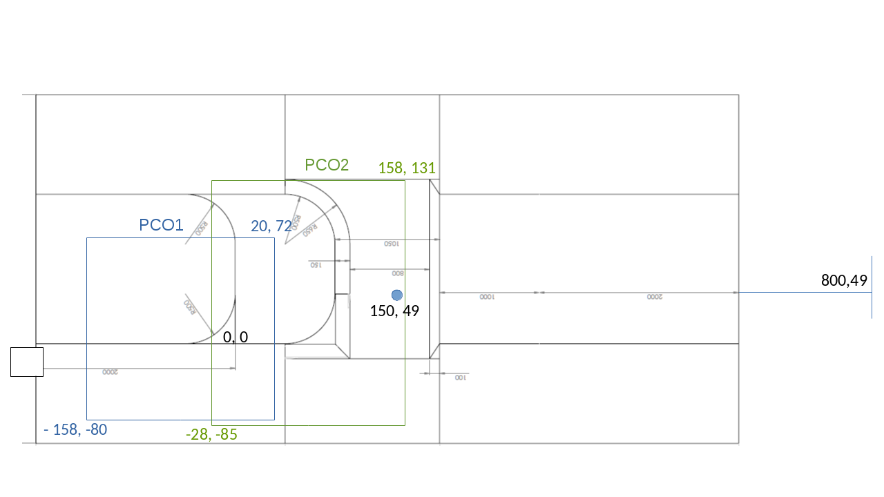
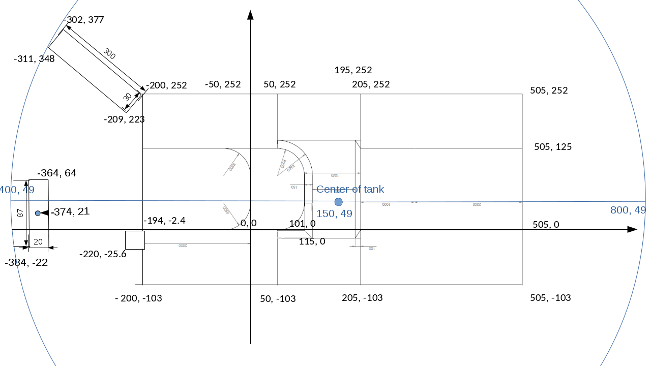
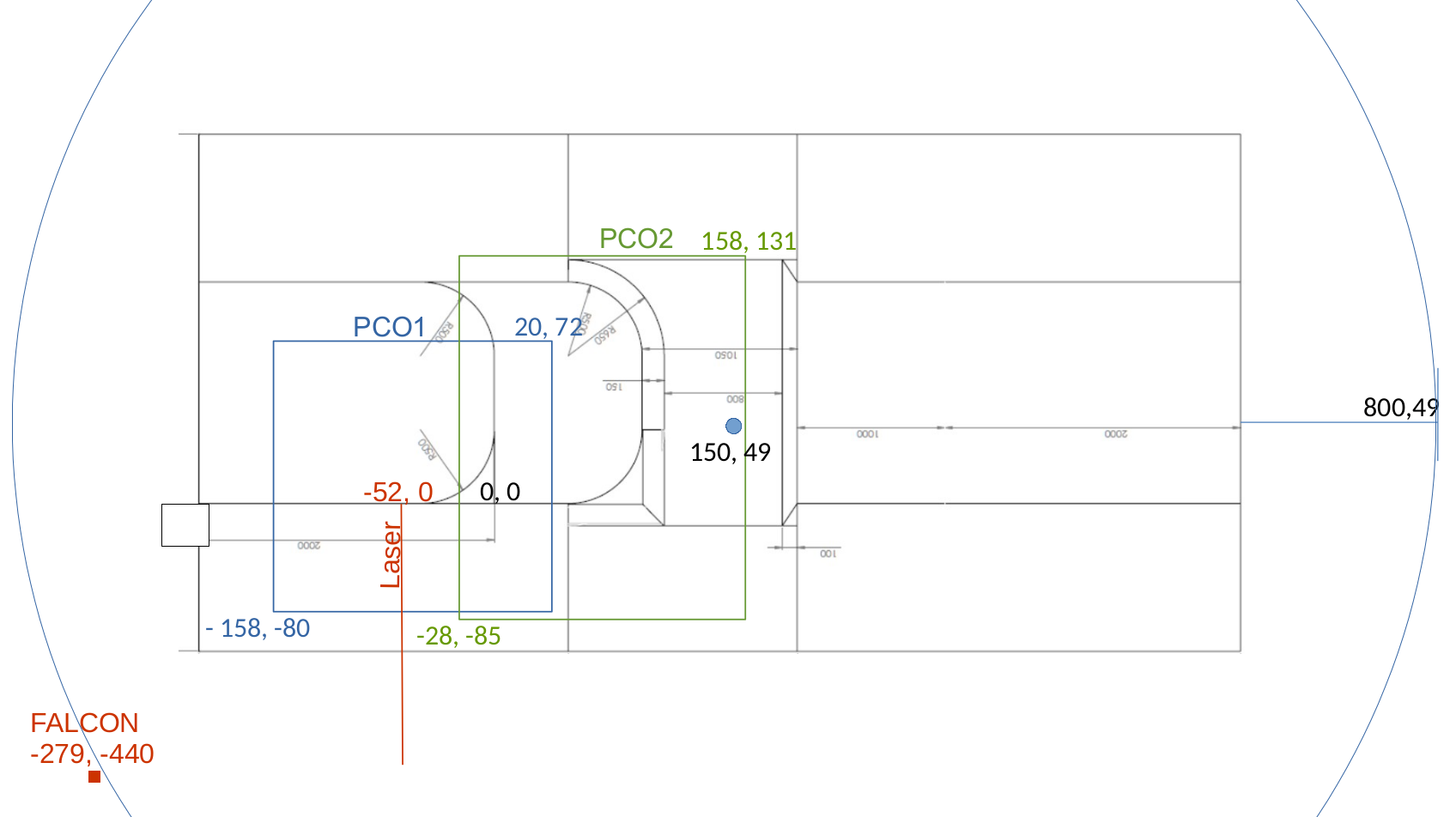
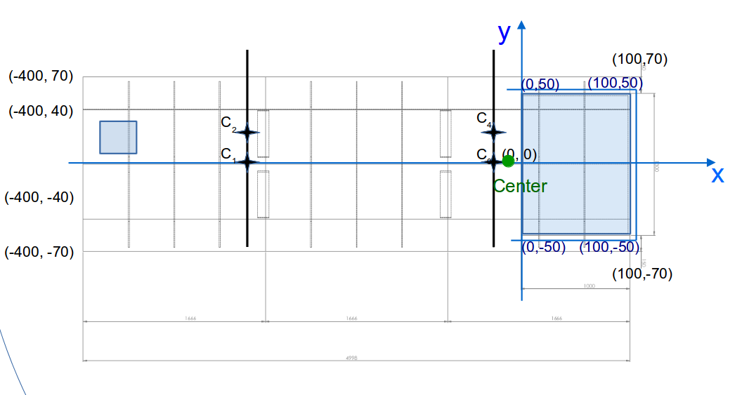
Sketch of the topography seen from above with the distances to the (0, 0) coordinate. The blue circle and the blue line are the tank wall and the centerline, respectively.

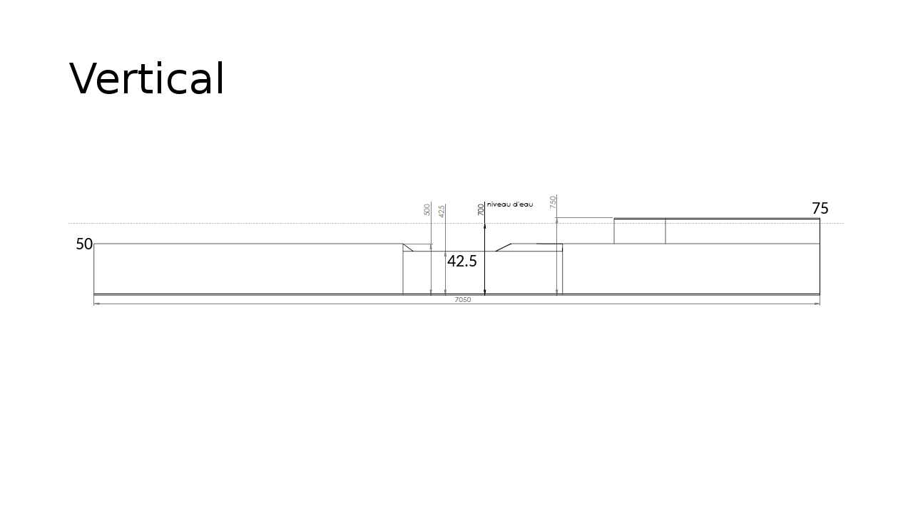
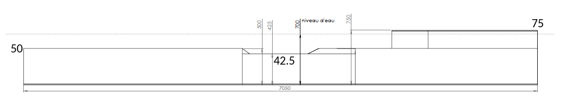
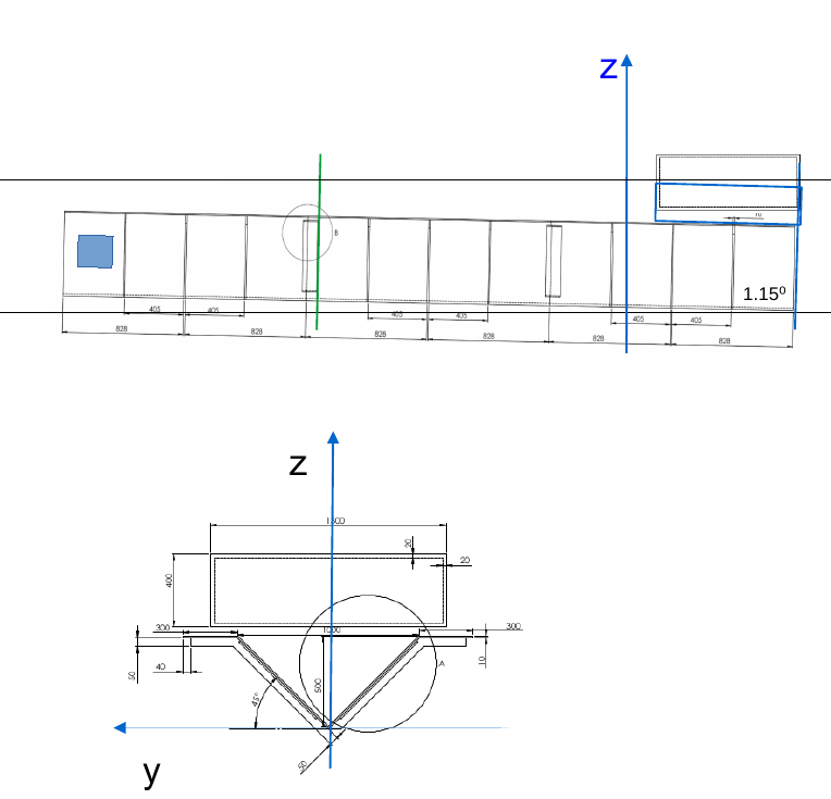
Sketch of the topography seen from the side with the heights of the different areas.
2.2.2 Topography for the ice shelf experiments
2.3 Reference axis
2.3.1 Reference axis for shelf break experiments
By definition we will use Ox and Oy axis to define the along slope and the cross slope axis. The central reference point (0,0) along the slope is chosen to be the first "land" corner downstream of the source. Positive u - direction corresponds to the along slope flow direction, while positive v - direction is directed onshelf. The position of the topography relative to this coordinate system is shown in 2.2.1
2.3.2 Reference axis for ice front experiments
2.4 References axis along the wall (horizontal and vertical) - Nadine add image!
By definition we will use Ox and Oy axis to define the along shore and the cross shore axis. The central reference point (0,0) along the wall is chosen to be the closest point to the center of the tank (also labeled M0?). Positive direction corresponds to the mean wave or the mean flow direction.
We use seven references points along the wall to quantify the impact of the free surface deformation and the possible vertical deviation of the laser sheet???

All these points will be measured every day before starting the Experiment??
| Position | M2 | M1 | M0 | M-1 | M-2 |
| H_coast (cm) | ' | ' | |||
| H_laser_up (cm) | ' | ' | |||
| H_laser_down (cm) | ' | ||||
2.5 Fixed Parameters
| Notation | Definition | Values | Remarks |
| $T_{rotation}$ | Rotation period | $50 \ s-1$ | |
| $H_{shelf}$ | Shelf height | $0.5\ m$ | |
| $H_{through}$ | Trough height | $0.42\ m$ | |
| $W_{trough-slope}$ | Width of slope in trough | m | |
| $s$ | slope | !1:2(Height:Width) | |
| $\nu$ | Viscosity | $10-6m2s-1$ | |
| $L$ | Total length of the wall | $ \ m$ | |
| $W_{Source}$ | Width of source (inner) | $ 23\ cm$ |
2.5 Variable Parameters
| Notation | Definition | Unit | Initial Estimated Values | Remarks |
| $H_{water}$ | Total water depth | $cm$ | 60 - 70 | At the point where waterlevel is not influenced by rotation: r=?? m. |
| $H_{shelf}$ | Depth on shelf | $cm$ | 10 - 20 | estimated where? |
| $R_c$ | Radius of curvature | $m$ | 0 - 0.5 | |
| $Q$ | Flux | $L min{-1}$ | 20 - ??- ?? - 135 | |
| $\Delta \rho$ | Density difference (ambient - inflow) | $kg$ | 0 - 3 - 10 |
2.6 Additional Parameters
| Notation | Definition | Unit | Initial Estimated Values |
| $g'$ | Reduced gravity | $m s{-2}$ | |
| $Rd$ | Baroclinic deformation radius | $cm$ |
2.7 Definition of the relevant non-dimensional numbers (UPDATE WITH OUR NOTATION!!)
Rossby number, $ Ro = U/W/f$.
Relative step size, $H* = \delta H/ (H-\delta H) $. (Cenedese et al, 2005)
Depth of baroclinic current ($H_{BC}=sqrt(2Qf/g')$ (Chapman & Lenz 1994; Sutherland et al, 2009)
Internal rossby radius ($\lambda_i = sqrt (g' H_{BC})/f$.
3 - Instrumentation and data acquisition
3.1 Instruments
Conductivity Sondes (CS)
Particle Imaging Velocimetry (PIV) A Spectra-Physics Millennia ProS 6W YAG continuous laser (532 nm) in conjunction with 2 cameras was used to provide PIV images. The laser light sheet was brought in parallel to the bottom of the tank. The light sheet can then be racked in the vertical through a series of steps through the use of a motorized traverse (tilted at 3.5 degrees to match the slope of the channel) and a mirror set at 45 degrees. The laser has another set of optics to point the light sheet down at the mirror, producing the light sheet. There is a glass window that enables the laser beam to go through the surface of the water tank. A 3D animation of the laser is in the ‘videos’ subfolder of the Photos folder. The laser light sheet positions are then synchronized with the PIV cameras. The field of view extends from close to the upstream end of the first bend, towards the mid-point of the second bend.
Later experiments used larger seeding particles, 200 micron polystyrene particles for the flow seeding. These work very well for these situations where the measurement area is larger than 2 square metres. The three PIV cameras consist of one Falcon1 camera (Falcon 4M, CMOS 2432*1728 pixels, 10 bits) over the upstream part – with a 35 mm objective lens, PCO2 over the first bend with a 35 mm objective lens, and PCO3 over the most downstream part of the PIV measurement area, which has a 20 mm objective lens. 15 slices in the vertical are taken, each containing 20 images and these are repeated 10 times. Four different times between frames are used, since the velocities were not known a priori and vary as a function of height in the gravity current. So as such, no specific frame rate is used. All this is in the .xml files which can be read by a text editor. The two PCO cameras are PCO.edge5.5 CMOS cameras (2560*2160 pixels). The general approach is to have the lowest slice at approximately 2 cm above the floor, and then there are 2.5 cm heights between each successive level. These varied over time however, so there are a number of slightly different setups – see below. The sequence starts at the highest point, and then steps down through the flow, to the bottom, before switching back to the top again. Heights of laser slices (22/09/16 – 2.5 cm but after that 12/10/2016 and 14/10/2016 and 19/10/2016 all at basal 2 cm).
3.2 Definition of time origin and instrument synchronisation
3.3 Requested final output and statistics
Batch processed camera data in to .png files for those experiments from 18-43 that have PIV data, so that images are in a non-proprietary format. PIV analysis of the flow field through multiple horizontal slices in different Z-positions, for the non-rotating case, and for the rotating cases (experiments 18-43 as above), dependent on the quality of the captured PIV images. Average velocity vectors for the channel slices. Potentially information on vorticity would enable the smaller-scale vortical structures that are obvious in some of the videos, to be identified.
4 - Methods of calibration and data Processing (NADINE)
The PIV data will be processed using the MATLAB tool UVMAT available on http://servforge.legi.grenoble-inp.fr/projects/soft-uvmat.
All images from the experiments will be stored in the directory /fsnet/projects/coriolis/2017/17ICESHELF/DATA under the name for the experiment.
4.1 Calibration for shelf break experiments
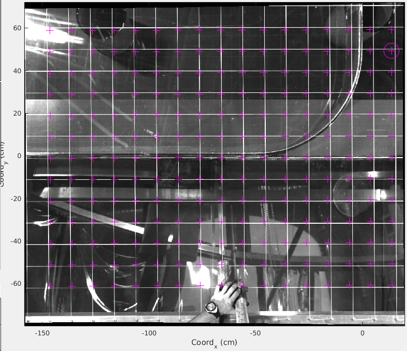
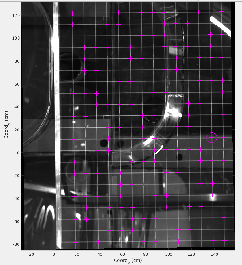
The images for PIV (PC01, PC02) are calibrated from images of a horizontal grid, in 3D with an inclined grid (tilted angles) and in the vertical (NAME OF CAMERA!) for the camera fixed on the tank wall.
The calibrated images with the grids are stored in 0_REF_FILES with the
- 2D calibration in the directory CALIB_07_09
- 3D calibration in the directory CALIB_07_09_3D
- Vertical calibration in the directory CALIB_VERTICAL_08-09
The images are divided into the two different cameras as PCO1/ and PCO2/.

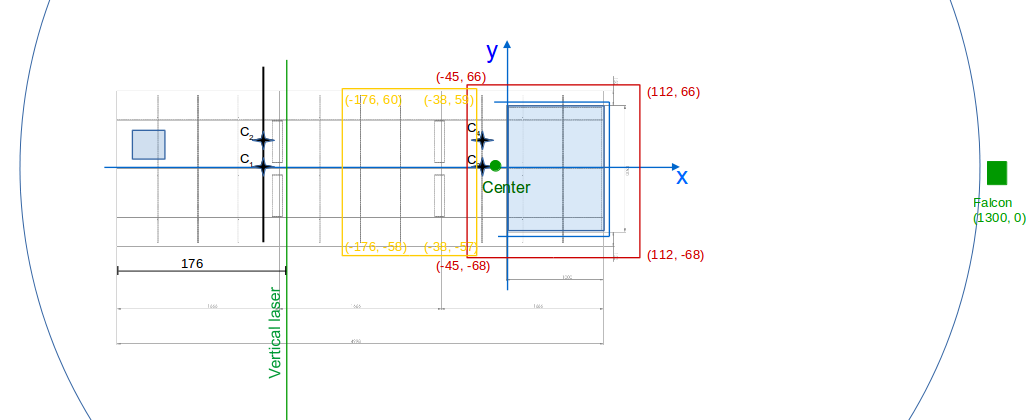
This sketch shows the topography together with the view of the two cameras.
The 3D calibration is done with the geometric calibration function on UVMAT to create 'intrinsic parameters' for each camera that will be used for all images. Calibration points along the inclined grid are marked and translated from image coordinates to physical coordinates defined in section 2.3.1 to later take into account the different height of slices. See http://servforge.legi.grenoble-inp.fr/projects/soft-uvmat/wiki/UvmatHelp#GeometryCalib for details of the method. The calibration parameters are copied in a xml file beside the folders of each camera (for instance PCO2.xml for PCO2/). The xml files also containing all the timing information and have to be copied next to the folders of all images, to use the same intrinsic calibration data for each image taken with the corresponding camera.
The 2D calibration is used as a reference horizontal grid with a grid height of
- z = 80.8 cm for PCO1
- z = 58.2 cm for PCO2


Calibration of camera 1 (PCO1) on the left and of camera 2 (PCO2) on the right, with the calibration grid produced with PIV in purple.
The calibration is checked with a calibration ruler (images saved in CALIB_RULER) to see that the transition between the two cameras is smooth.
For the vertical calibration the images are saved in a different file format with extension '.seq'. The format can be changed in the UVMAT software, but the folder with the vertical images should not be renamed (e.g. '2017-09-08T16.04.32'). To change the image format, choose RUN -> Field Series. Chose the right input file, an select 'extract_rdvision.m', click INPUT and RUN. The image will be saved in a new folder as a .png file and is ready for use in UVMAT.
4.2 Calibration for ice shelf experiments
5 - Good to know…
5.1 How to turn on and off the lasers

The laser for horizontal slices is turned on and off in the rotating office via the computer. You only have to switch the shutter between on and off.

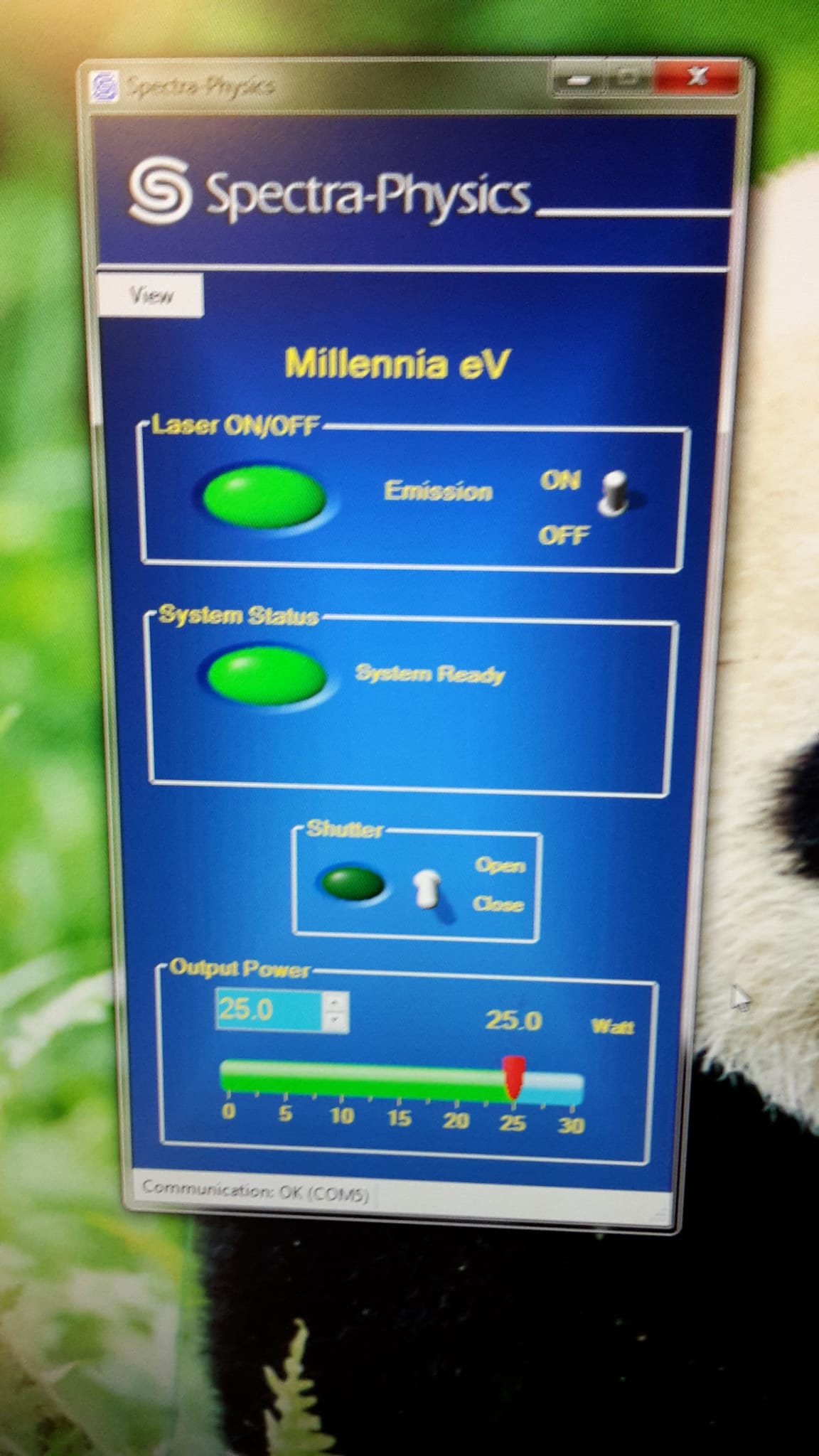
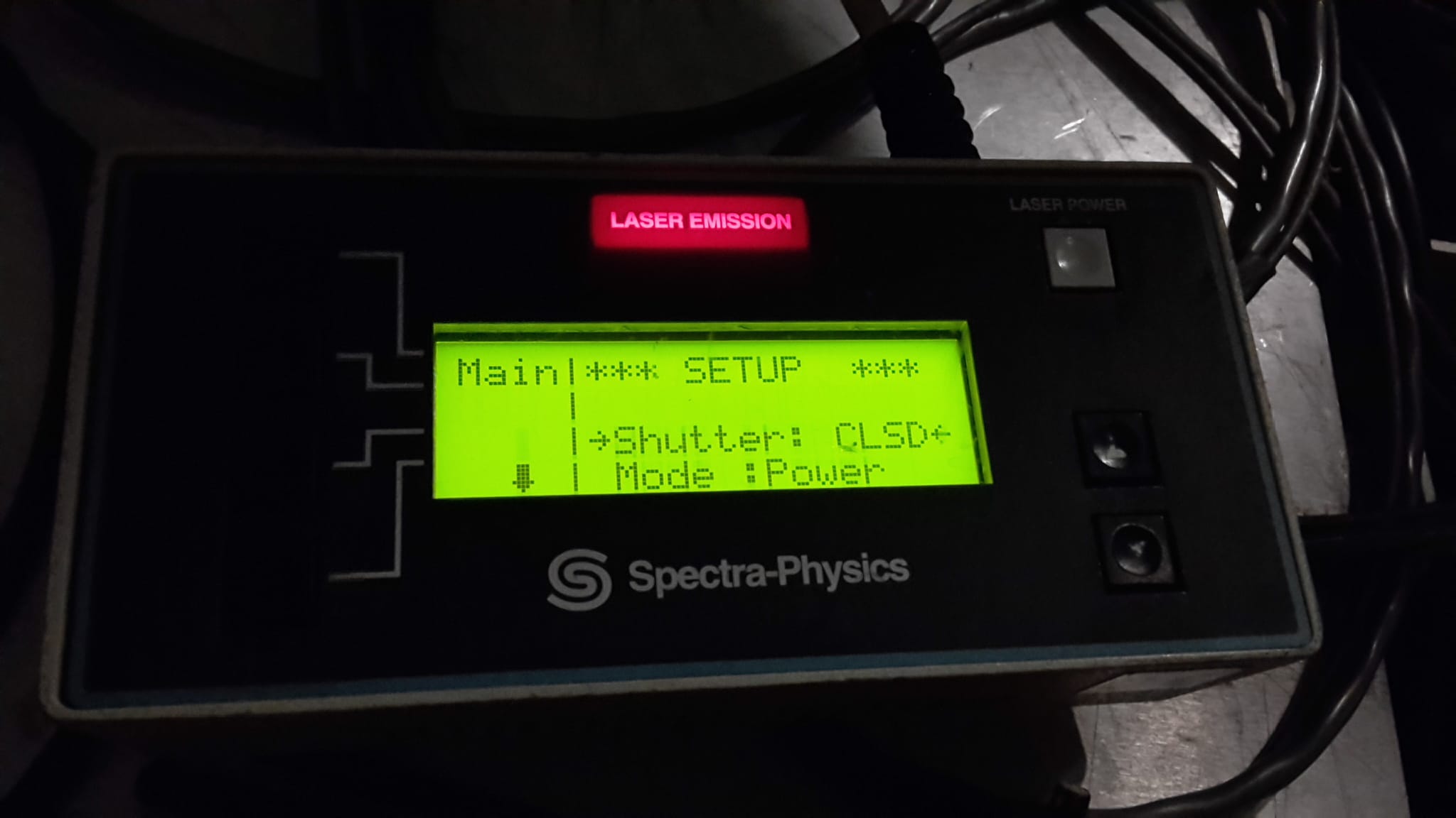
The laser for the vertical slices is turned on and off outside the wall, where the laser is located. Press the button in the lower right corner of the instrument in the photo.
6 - Organization of data files
All data related to the project are in:
SERVAUTH4\share\project\coriolis\2016 or
servauth4.legi.grenoble-inp.fr\share\project\coriolis\2016
- 0_DOC: miscellaneous documentation and reports
- 0_MATLAB_FCT: specific matlab functions
- 0_PHOTOS: photos of set-up
- 0_PIV
- Each ‘PIV’ folder contains subfolders for each of the 3 PIV cameras: Dalsa (sometimes Falcon1 – it’s the same thing); PCO2; PCO3 [these are named after the different brands of camera]. Other folders include PCO2.png and PCO3.png which contain processes images of the PCO cameras that are in a non-bespoke format. Other folders that can be within the Camera folder include: Dalsa.sback; Dalsa.sback_1; PCO2.png.civ; PCO2.png.civ_1; PCO2.png.civ_2; PCO2.png.sback: PCO2.png.sback_1; PCO3.png.sback_1. .sback files refer to those files where the background has been subtracted, then civ_1 contains images with the first PIV iteration as processed in UVMAT (Joel’s code) and shows the raw data – with or without the rejected vectors; vectors are shown in four colours, blue = best, green = medium, red = poor, and pink = false. A box can be clicked to hide the false vectors. Civ_2 uses a spline interpretation to interpolate between vectors, so long as they are close enough to the surrounding vectors. Then interpolates all the vectors onto a regular grid. Times for the .png images are in the XML files, or netcdf files.
- 0_Processing: UVP processing scripts in Matlab
- 0_REF_FILES: files of general use (calibration data, grids ...)
- EXP1, EXP2, folder for each experiment with names given in the table below. The names refer to ‘fix’ for non-rotating fixed case, ‘rot’ for rotating case, ‘str1’ for the first straight position (also called position X1), and ‘apex 2’ , for the apex in bend 2 (also referred to as position X4).
- Within each experiments, there is a folder with PIV imagery called ‘Camera’, one for ADV data – ‘ADV’, one for UVP data – ‘UVP’, and one for the data coming directly off of the Coriolis table control system ‘LABVIEW’. Some experiments also contain an ‘Images’ folder or a ‘Gopro folder’ containing Gopro videos.
- Each ‘Camera’ subfolder contains subfolders for each of the 3 PIV cameras: Dalsa (sometimes Falcon1 – it’s the same thing); PCO2; PCO3 [these are named after the different brands of camera]. Other folders include PCO2.png and PCO3.png which contain processes images of the PCO cameras, that are in a non-bespoke format. Other folders that can be within the Camera folder include: Dalsa.sback; Dalsa.sback_1; PCO2.png.civ; PCO2.png.civ_1; PCO2.png.civ_2; PCO2.png.sback: PCO2.png.sback_1; PCO3.png.sback_1
- Each ‘ADV’ subfolder, contains two sub-folders: ‘nkt_files’ containing raw Nortek files, and the ‘mat_files’ are the exported raw data in Matlab format.
- Each ‘UVP’ subfolder contains two folders – one with the experiment name (which is the downstream velocity data) recorded downstream of the velocity inflection downstream of bend apex 2, and one with experiment name ‘_cross’ which contains the cross-stream UVP data recorded at bend apex ‘2. These two folders contain text files for each of the probes. The convention is that Probe 1 is the basal probe, with each subsequent probe being successively higher. There are also .mfprof files which are the raw UVP data in native format. All probes are also integrated into single Matlab files. Lastly, there is a Logfile with the header file for the UVP detailing all of the parameters used in the run.
- Each ‘LABVIEW’ subfolder contains: 1) a .lvm file which is a text file and contains a time-stamp, two voltages for the Conductivity probe on the traverse (C0 – Conductivity, and T0 – temperature [this latter one doesn’t work]), a Trig_cam heading representing the Trigger for the PIV Cameras, Conductivity probe in the input box (C1 and T1), and C2 (this was conductivity for a second probe in the input box which was briefly used before breaking. There is always a record for this but it is just background noise. 2) _position.lvm file which is an XYZ file with a times for the movement of the traverse. 3) Some folders also contain probes.nc files. These are netcdf files and contain the vector data from the processed PIV images.
- Within each experiments, there is a folder with PIV imagery called ‘Camera’, one for ADV data – ‘ADV’, one for UVP data – ‘UVP’, and one for the data coming directly off of the Coriolis table control system ‘LABVIEW’. Some experiments also contain an ‘Images’ folder or a ‘Gopro folder’ containing Gopro videos.
7 - Diary:
7.1 Thursday 07 September
The cameras still have to be adjusted. After that is done, we take photos with the calibration grid in the horizontal and in 3D with both cameras that are fixed on the roof. With PIV, we conduct the calibration of both cameras as described in 4.1.
7.2 Friday 08 September
To verify the calibration, we took photos with both cameras with one ruler to see if the calibrations of the cameras agree (which it does!). Then, we added a wall into the tank to prevent the water of the freshwater experiments to return to the source. The laser height was adjusted.
7.3 Monday 11 September
The table starts rotating for the first time with a velocity of 50 rounds/ sec. It gets slowly filled with water to a level of 60 cm. This takes about 3h.
After filling the tank Thoma measured the water level to be point where water level does not change with rotation 60.4 cm Center of tank – 42.5 + 16 cm = 58.5 cm Tank wall (6.5 m) – 62.4 cm. Water temperature 23.3C.
Particle sedimentation test : Water was taken from the tank, mixed with particles (30 + wetting agent) and set to settle in a glass “vase” with a narrow (ca 3cm) and tall (ca 10 cm) neck. The upper level with particles were observed as follows:
| Time | level |
| 11:50 | 0 |
| 13.05 | 4 mm |
| 13.30 | 5 mm |
At 14h40 the border was now longer visible. There were still particles in the upper part of the flask, but a lot less than there were intitally.
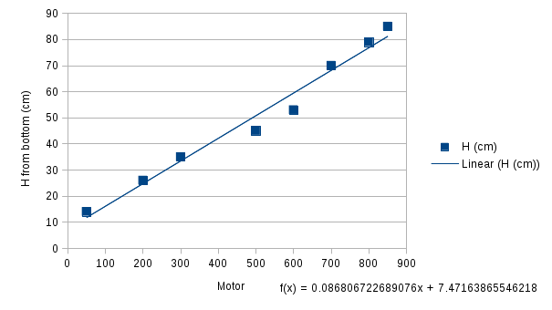
Calibration of vertical laser sheet
While changing the settings on the laser, the actual height of the laser sheet was measured directly in the tank.
| Laser setting | $H_{real} | |
| 650 | 55 cm | |
| 700 | 49.5 cm | |
| 800 | 40 cm | |
| 850 | 35 cm | |
| 900 | 30 cm |
We will use 650 :50: 900 to get Slices every 5 cm from 30 cm to 55 cm (total 6 Slices).
TEST experiments
The desired flow rate of 50 L/min should according to 0_DOCS\flow_rate.xclx should be achieved With a diaphragme of diameter 12.9 mm. We used 13 mm. The flow rate was estimated by measuring the time it took for the water Level in the feeding tanks to descend from 170 to 150 (with the pumps turned off) - it took 41s giving a flowrate of 40 L / 41 s = 58.5 L/min.
The pipe was first opened to remove boubles from the system. The Sources was designed in a way that the hose stopped just below the top of the Source which was out of the pater, thus creating a small waterfall, turbulence and a lot of boubles that got throught the honeycomb and flowed along the slope With the current. The Source will be redisgned so that the water is inserted below the water surface.
A second trial (still with the original source) was made later (when Samuel was back). The same ddiaphragme was used and the same amount of boubles was created. Flourescent dye (NAME) was injected first in the feeding tank above, then in directly in the water just upstream of the vertical laser sheet.
Time series of photos was obtained from the vertical camera.
Aperture 150ms Time between photos 450 ms.
There were more particles in the inflow than in the ambient, and the border between the inflow and the ambient was seen to fluctuate up and down the slope. The timescale of this motion will be estimate from the photos tomorrow.
When turning to the horizontal cameras it was decided that sloping topography gave too many uncontrolled reflections that made it unsafe to increase the intensity. To remove these,parts of the bathymetry has to be Paint in black. The tank was set to empty during the night, while recycling the water.
7.4 Tuesday 12 September
The bathymetry has been painted black, a pipe has been introduced into the source and the drain has been lowered to that it can be used also for 60 cm water depth.
The tank is filling: $T_{water}=22.9C, \rho=998.5 kg m^{-3}, T_{air} = 23C$.
The reflection is now ok and we can start our experiments!
Test experiment EXP01
We conducted experiments with a long HS from the beginning after turning on the influx (EXP_01). The influx was 41 L/min with a diaphragma of 12.6 mm diameter. The influx water had a density of 998.2 and was enriched with particles of size 30mikrom. The laser sheet was at 11cm over the trough, 4 cm over the shelf, so at 54 cm when the laser setting was at 650. We decreased it to 640 to have the laser sheet at 55 cm. Water Level (supervision - this changes witha few mm when People come enter/leave the rotating Office) was at 58.4 cm. The exposure time of the cameras was at 50ms and the time interval 500 ms.
We switched to the VS at 14:58 (EXP01_VERT).
terwards we started the Scan at 15:15 (EXP01_SCAN) with the same camera settings as for the HS. The slices were at the heights of 55 cm to 30 cm in 5 cm steps. We took 4 images at each height with a time interval of 500 ms.
Observations: On the horizontal scans we can clearly see turbulent/vertical motion along the coast. They turn left at the curvature and follow along the topography to the wall. Some particles turn right above the trough/ shelf and flow out to the slope again.
Data check: We checked these first results with the PIV and decided to decrease the exposure time to get sharper images of the particles. With PCO2, the flow around the curvature can be captured with the PIV, but on PCO1 the PIV is not very good, because the flow is more turbulent and more 3 dimensional. We decide to decrease the time between the photos. Later we realized that the cameras only took every second photo, so with a time interval of 1000ms - > useless PIV.
Experiment EXP02
We repeated the HS with a reduced time to 200 ms between the photos and and exposure time of 30ms. We realized afterwards that the cameras only took every second photo, so with a time interval of 400ms!
7.5 Wednesday 13 September
The cameras are fixed now and taking every photo and the particles are spread out in the ambient water.
Experiment EXP03
The setup is still the same as for the previous experiments with 200ms time difference between the photos (this time working!) and particles in the ambient water. This time, we measured the flow rater AFTER the experiment and it was $Q = 50 l/min$ (measurements repeated twice), as expected. There are still bubbles coming out of the source!
The current reached the first corner after about 1 minute, and the trough corner after about 3 minutes.
Experiment EXP04
We started a new experiment at !10:31 with a reduced flow rate of about $Q = 20 l/min$ (diaphrama diameter of 6.8 mm). The first HS is run for 15 min n(!10:31- !10:46). The flow field was still evolving so we extended the five more minutes of hs (!10:51-10:56 this data are stored in EXP04_B) before we started the scan ( !10:59).
Note: During the scan, the laser is shaking too much! This needs to be changed.
Observations: The bubble at the source disappeared due to the lower flow rate. The current follows along the slope and turns left at the 2nd curvature into the trough. After the 15 min after the flow was turned on, the flow bifurcates at the continental coast and at the trough and fills up the trough. The return flow does not follow along the upstream slope of the trough, but occurs in the middle of the trough. The main current along the slope is getting wider with time.
Experiment EXP05
The vertical velocity of the laser was decreased and the timestep between the first and the second image at each level increased to 1s (first image will be discarded).
The tank from where the inflow is pumped was mistakenly filled with too much Cold water (T=19.2C) - i.e. about 4 c colder than the water in the tank.
There where a lot of Bubbles coming out from the Source - and we observed large (10 cm) airbubbles travelling Down the hose during the Experiment.
All the water turned at the first water, onto the shelf.
The current was at the first corner about 1 minute after the valve was opened.
Experiment EXP06
The squared cornes were inserted - the land corner was fastened with tape and the submerged corner with a screw..
To reduce to amount of Bubbles coming out from the Source we added a thin sheet of foam behind the honey comb. In addition, the joints of the tube where the diaphragm is inserted was greased. This appeared to help - the amound of Bubbles was greatly reduced and no Bubbles was seen travelling Down the hose.
The flow separated at the first corner and turned at the second corner.
The vertical scann was started 15 min after the valve was opened.
Experiment EXP07
An eddy initially forms behind the first corner, but it then disappears.
The flow turns into the through. Large eddy on the Continental shelf (as in Kjerstis model Experiments!).
When scanning dt was set to 100 ms, but only every second photo was aquired so dt= 2 x 100.
7.6 Thursday 14 September
Experiment EXP08
The squared corners are still on, for the first 3 minutes of the horizontal slice the light in the entrance was turned on.
The flow turned left at the second corner following the slope in the depression keeping a "tight" shape on the topography.
After a while, a straight flow established, following the slope. The circulation is very slow compared to yesterday.
For the scan there is dt =1000ms between the first and the second image at each level, then dt=400ms. First image is not used to PIV
This is to avoid shaking of laser.
Experiment EXP09
The squared corners are removed and the flow rate is reduced. There were a lot of particles in the inflow in the beginning.
There is a clear split of the flow at the 2nd corner, the main part crosses the depression following the slope and a much smaller part followed the topography inside the depression.
The laser sheets were started 26 minutes after the valve was opened.
Experiment EXP10
The flow rate is increased, there are again a lot of bubbles.
Time to reach the first corner: less than 1minute.
After the reaching the first corner a major part of the flow followed the boundary and circulated on the shelf.
A smaller part continued to the corner of the slope and the depression (after 3minutes) and entered the depression, circulated along the topography and escaped by the western side of the depression
Experiment EXP11
The water level is increased by 10 centimeters to 68.5 cm. With the higher water level, we need to calculate new flow rates with the ration of the outflow area before and after the higher water level. Now, we are aiming to a flow rate of 33 l/min, which corresponds to the 20 l/min for the lower water level.
Conversion of flow rate from low to high water level:
| Q (low water level) | Q (high water level) |
| 10 | 17 |
| 20 | 33 |
| 35 | 58 |
| 50 | 83 |
| 80 | 133 |
Note: In the previous experiment, the measured flow rate was always higher than the expected one with their diaphragme - flowrate curve. We plotted the diaphrame vs. flowrate again with the values from our experiments. For the flowrate of Q = 33 l/min, we therefore used a diaphragme with diameter of 10 mm, instead of 8.6 mm (which it was for the 20 l/min flux before).
We measured the flux 4 times during this experiment. It gave:
- 32.4 l/min
- 34.5 l/min
- 33.3 l/min
- 34.9 l/min
Measured water level after the experiment: 72.7cm at the edge and 68.5cm over the topography.
Time to reach the first corner: 3 min.
Observations: There are no more bubbles. The flow crossed the shelfbreak between the 1st and the 2nd corner. After the flow is established it follows along the rough topography and returns along the continental coast.
There was no straight flow along the slope.
There were very few particles in the end of the horizontal slice. On the vertical slice the flow does not look barotropic.
Note: After Exp11 they realized that there was water in the laser, they had to go and move it up.
Experiment EXP12
This experiment was the same as EXP11 with a water level of 68.5 cm but with the corner. The expected flowrate was 33 l/min and the measured flowrate was 34.6 l/min.
The exposure time was increased to 40 ms, because the flow is slow - so no need to have a short exposure time. It makes the particles more visible.
7.7 Friday 15 September
Experiment 13
During night, we increased the rotation rate to get a rotation period of 30s! We kept the corners.
There were still many particles in the ambient water, but Thomas sprayed more particles on the surface.
New measured water levels:
- wall: 69.8 cm
- center: 59.5 cm
- invariant: 65 cm
Water level on the screen: 63.4 cm
For the desired fluxrate of 50 l/min, we used the diaphragme with 12.6 mm diameter. The measured fluxrate after the experiment was 54.5 l/min.
Observations: In the beginning of the experiment, there were too many particles in the influx, but got less with time. The main current turned left at the second corner into the trough.
Note: The source is leaking, which created bubbles and a little "waterfall" due the the water surface difference inside and outside the source. Thomas fixed it by putting a wooden block in front of the leakage.
Experiment 14
We increase the influx to a desired value of 80 l/min with still the higher water level and increased rotation rate.
Due to the high flux rate, we use an exposure time of 30 ms.
Notes: The water level increased constantly. After this experiment, we had to adjust the sink to let out more water. It takes some time, so we had to wait until the water level was good again.
' 6 - Table of Experiments:
- will be updated from Excel sheet!
| Exp No. | Name | Valve opened | $H_{water}$ | $T_{rot}$ | $Q$ | $R_{curvature}$ | $\Delta \rho$ | Diaphragme | Flowrate estimated | Type of photo | Height of HS | Heights of Scan and # | Time photo | Dye | Comments | Notes |
| $(m)$ | $(s)$ | $(L min^{-1})$ | $(m)$ | $(kg m^{-3}$ | $(mm)$ | $H_1,H_2,\Delta t $ | VS/HS/Scan | $cm$ | $cm$ | t1/t2/t3 $\Delta t$ | yes / no | |||||
| 0 | test | 11092017 hh:mm | 0.604 | 50 | 58.5 | 0.50 | 0 | 13 | 170,150,41s | VS | - | - | ? | yes | Dye did not show up in photos :-( | Elin |
| 1 | exp01 | 12092017 !14:38 | 0.584 | 50 | 40.67 | 0.50 | 0 | 12.6 | 170,150,59s | HS,VS,Scan | 55 | 55:[-5:30,4 -5:30;4] | 500ms (reality: 1000ms) | no | Expl. time = 50 ms too little. Only every second photo was taken | Elin |
| 2 | exp02 | 12092017 !17:02 | 0.583 | 50 | 44.2 | 0.50 | 0 | 12.6 | 180,150,81.4s | HS | 55? | - | 200ms (reality: 400ms) | no | Only every second photo was taken | Elin |
| 3 | exp03 | 13092017 | 50 | 50 | 0.50 | 0 | 12.6 | HS,Scan | 200ms | no | Problem with photos fixed; particles in ambient | Elin | ||||
| 4 | exp04 | 13092017 | 50 | 0.50 | 0 | 6.8 | HS,Scan | 200ms | no | Laser started vibrating for the scans | Elin | |||||
Attachments (18)
- DSC_0811_00001.jpg (59.5 KB) - added by 9 years ago.
- PCO1_Calibration2.png (437.0 KB) - added by 9 years ago.
- PCO2_Calibration.png (368.8 KB) - added by 9 years ago.
-
Bathymetry_with_PositionCameras.pdf (47.4 KB) - added by 9 years ago.
Topography with the positions of the cameras
-
Bathymetry_with_Positions.pdf (56.7 KB) - added by 9 years ago.
Topography position relative to the tank walls with source
- Topography_with_PositionCameras.png (57.9 KB) - added by 9 years ago.
- Bathymetry_with_Positions.png (107.4 KB) - added by 9 years ago.
- Bathymetry_Vertical.png (25.3 KB) - added by 9 years ago.
- Bathymetry_Vertical.2.png (25.3 KB) - added by 9 years ago.
- Bathymetry_Vertical.3.png (25.3 KB) - added by 9 years ago.
- Bathymetry_Vertical.4.png (10.0 KB) - added by 9 years ago.
- horizontallaser_switch.jpg (193.0 KB) - added by 9 years ago.
- verticallaser_switch.jpg (96.2 KB) - added by 9 years ago.
- Bathymetry_with_PositionCameras.png (118.9 KB) - added by 9 years ago.
- Conversion_MotorLevel_LaserSheet.png (15.5 KB) - added by 8 years ago.
- Channel_Sideview_with_Coordinates.png (57.7 KB) - added by 8 years ago.
- Channel_with_Coordinates.png (60.8 KB) - added by 8 years ago.
- Channel_with_CameraPositions.png (42.7 KB) - added by 8 years ago.
Download all attachments as: .zip