
| Version 9 (modified by , 13 years ago) (diff) |
|---|
This is an example using more advanced tools than the examples .... and .... Image pre_processing and merging of mutiple fields. Open the example UVMAT_DEMO_FILES/EX07_convection .
calibration
mark corners
mask
sub_background
first PIV
making two masks
The parietal jet requires a very good resolution, particularly among x. To limitate PIV to this jet, let us create a specific mask. Open the previously created contour polygon contour_mask.xml in uvmat by the menu bar Tools/Projection object/browse.... Check the box edit (tag [CheckEditObject]) in the frame Object of uvmat (right hand side) to allow editing of the polygon. then replace the lower x bound 0 by 52. Then create the corresponding mask by Tools/make mask, save it with name Dalsa1.mask/mask_plume.png. Similarly create a mask for the bulk Dalsa1.mask/mask_bulk.png, with bounds in x [0 55].
PIV on the parietal plume
Choose the following parameters:
- pair j=1-2 for Civ1 and Civ2 : it minimises the time interval which is needed to capture the large velocity in the plume.
- CorrBox x,y=(5 31) which optimizes the resolution in x (5 pixels)
- Search x, y=(25 55) which allows for a larger velocity component along y .
- auto-grid Dx=2, Dy=10, consistent with CoorBox (about half the box size).
- Mask selected, with name .../Dalsa1.mask/mask_plume.png .
- For Civ2, same parameters CorrBox, auto-grid and Mask.
- For patch and Fix, default parameters.
PIV on the interior
Select the pair j=1-3 to deal with the small velocities (considering that the parietal plume has been masked). Then use the default parameters.
merging data on a common grid
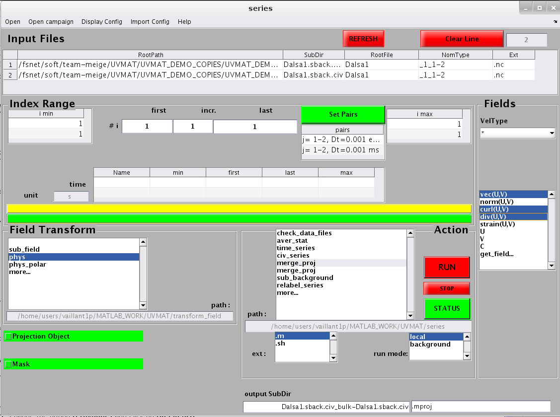
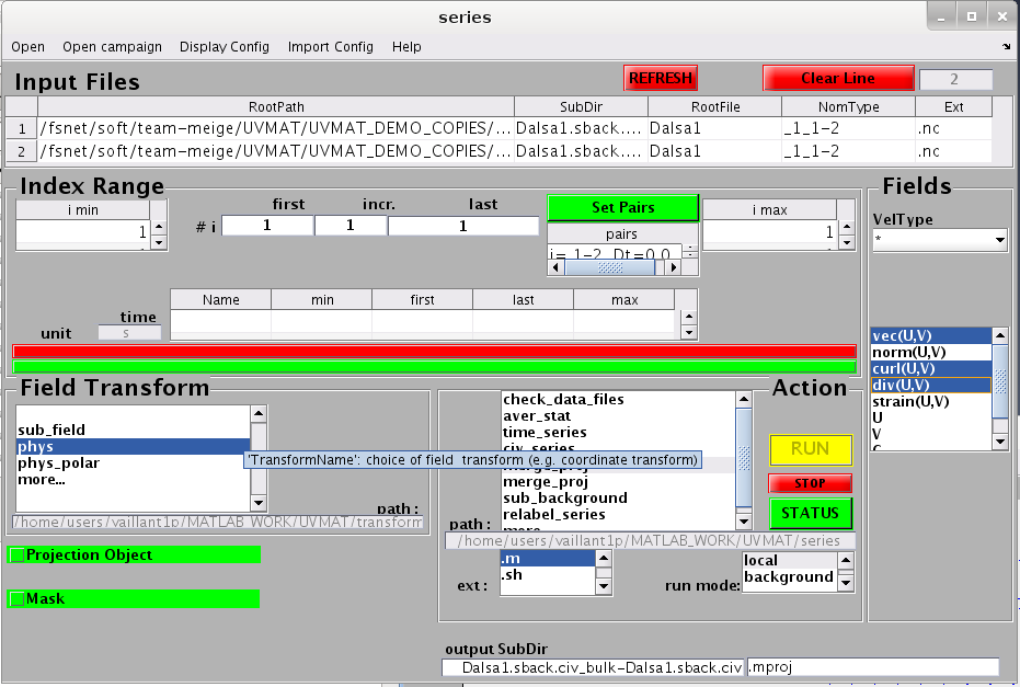
create a projection grid in phys coordinates. For that open a velocity field with uvmat, displayed in phys coordinates. Use the upper bar menu option Projection object/plane. Then in the GUI set_object, choose the option ProjMode=interp_lin. Choose a mesh 0.2 cm in each direction, ranging from 0 to 58.8 in x and 0 to 55 in y. Press REFRESH to see the result of projection in the GUI view_field. Check the option nb_vec/4 to reduce the number of vectors displayed on the plot. Now in series open the PIV file Dalsa1.sback.civ_bulk as input. Then append the second file Dalsa1.sback.civ_plume using the menu bar selection Open/Browse? append.... Set FieldTransform? to 'phys', and selection Projection Object. The plane is then incorporated in series.
Attachments (2)
- Tutorial8 - Merging data using thin plate spline.png (68.2 KB) - added by 11 years ago.
- Tutorial8 - Merging data using TPS.png (65.4 KB) - added by 11 years ago.
Download all attachments as: .zip