
TracNav
- Tutorial8: Correlation Image Velocimetry: advanced features
- Tutorial1: Image display
- Tutorial2: Projection objects
- Tutorial3: Geometric calibration
- Tutorial4: Processing image series
- Tutorial5: Correlation Image Velocimetry: a simple example
- Tutorial6: Correlation Image Velocimetry: optimisation of parameters
- Tutorial7: Correlation Image Velocimetry for a turbulent series
- Tutorial9: Image Correlation for measuring displacements
- Tutorial10: Image Correlation for steroscopic vision
- Tutorial11: Correlation Image Velocimetry with 3 components
- Tutorial12: Comparaison with a Numerical Solution
Tutorial / Advanced Particle Imaging Velocimetry
This is an example using more advanced tools than the simple example Tutorial: Particle Image Velocimetry. Image pre_processing and merging of multiple fields is used to optimise PIV in the case of a narrow parietal jet (produced by convection in a cavity). Open the example 'UVMAT_DEMO6_PIVconvection/Dalsa1' (accessible on http://servforge.legi.grenoble-inp.fr/pub/soft-uvmat/).
Calibration
Perform the geometric calibration by selecting the four box corners with the mouse, as described in Tutorial: geometric calibration, section 'calibration with reference points'. Alternatively, you can skip this operation by using the reference file 'Dalsa1.ref.xml' provided, removing the extension '.ref' to make it active.
Mask
Open the original image with uvmat, selecting the transform option 'phys'. Create a mask polygon by the menu bar command [Projection object/mask_polygon]. Set the option 'mask_outside' and introduce the coordinates of the four corners in [Coord] (like for geometry_calib). Plot the polygon, save it as 'contour_mask.xml' then create the corresponding mask by [Tools/make mask]. The default name is 'mask_1.png' in the subfolder 'Dalsa1.mask'.
Sub_background
We observe parasitic light rays on the images which correspond to fixed features, leading possibly to spurious velocity vectors equal to 0. To eliminate those we use the [Action] function 'sub_background'. In the GUI uvmat, select [Run/field series]. Then select the program 'sub_background'. This function is not provided in the default menu, so you need to use the last menu option 'more...', and select the function in the sub-folder 'series/' of the package uvmat. This option is then preserved in the menu for later use. Then [RUN] 'sub_background' over the whole index range in i and j, using the default parameters. Answer [Yes] to the question 'apply levels', which will conveniently rescale the image brightness after background removal.
First PIV
Do a PIV on the whole image series, optained with 'sub_background' (stored in a 'Dalsa1.sback' subfolder), selecting all the options from [CIV1] to [PATCH2] (see Tutorial: Particle Image Velocimetry for an introduction).
Choose the pair 'j=1-2' which provides the smaller time interval (100 ms), a good choice to capture correlations in a first try (although higher precision can be obtained with a larger time interval if the correlation is still of good quality).
Select the check box [Mask] and open the file 'mask_1.png' previously created.
Looking at the results with uvmat, we see the global flow features. We notice however that the thin parietal plume is not properly resolved while the precision in the interior is poor because of the small displacement within the frame pair. So the next step will be to perform two PIV series optimized for each sub-region and merge them.
Making two masks
The parietal jet requires a very good resolution, particularly among x. To limitate PIV to this jet, let us create a specific mask. Open the previously created contour polygon 'contour_mask.xml' in uvmat by the menu bar [Projection object/browse...]. Check the box edit (tag [CheckEditObject]) in the frame [Object] of uvmat (left hand side) to allow editing of the polygon then replace the lower x bound 0 by 52. Select the [SAVE] button to save it as a .xml figure. Create the corresponding mask by [Tools/make mask], save it with name 'Dalsa1.mask/mask_plume.png'. Similarly create a mask for the bulk, saving it as a .xml figure and with [Tools/make mask] as 'Dalsa1.mask/mask_bulk.png', with bounds in x [0 55].
PIV on the parietal plume
Open an image of the subfolder Dalsa1.sback (for instance Dalsa1_1_1.png) and open the GUI series/civ_series. Choose the following parameters:
- pair j=1-2 for Civ1 and Civ2 : it minimises the time interval which is needed to capture the large velocity in the plume.
- CorrBox x,y=(5 31) which optimizes the resolution in x (5 pixels)
- Search x, y=(25 55) which allows for a larger velocity component along y .
- auto-grid Dx=2, Dy=10, consistent with CoorBox (about half the box size).
- Mask selected, with name .../Dalsa1.mask/mask_plume.png .
- For Civ2, same parameters CorrBox, auto-grid and Mask.
- For patch and Fix, default parameters.
- Make sure the images go from i=60 to i=150.
Select [OK] and in the GUI series change the name at the bottom [output SubDir] by 'Dalsa1.sback.civ_bulk'.
PIV on the interior
Select the pair j=1-3 to deal with the small velocities (considering that the parietal plume has been masked). Then use the default parameters to [RUN] the PIV calculation with the 'mask_bulk.png' mask.
Merging data on a common grid
Create a projection grid in phys coordinates. For that purpose, open a velocity field of 'Dalsa1.sback.civ_bulk' with uvmat, displayed in phys coordinates. Use the upper bar menu option [Projection object/plane]. Then in the GUI set_object, choose the option [ProjMode]='interp_lin'. Choose a mesh 0.1 cm in each direction, ranging from 0 to 58.8 in x and 0 to 55 in y. Press [REFRESH] to see the result of projection in the GUI view_field. Check the option nb_vec/4 in view_field to reduce the number of vectors displayed on the plot.
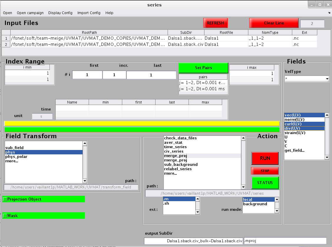
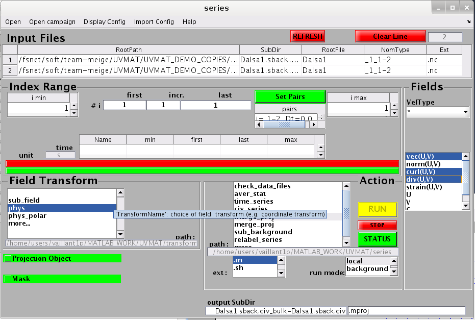
Now in series open the PIV file 'Dalsa1.sback.civ_bulk' as input. Then append the second file 'Dalsa1.sback.civ_plume' using the menu bar selection [Open/Browse append...]. Select [ActionName]= 'merge_proj'. Set [FieldTransform] to 'phys', and select the check box Projection Object. The plane for projection is then incorporated in series. It is also advised to introduce masks in the interpolation process so that each field is interpolated in its range of validity. This is done by selecting the check box Mask. Use the browser to fill the table of masks, in accordance with the order of the files in the table of input file series. Press [RUN] to launch the calculation. Then press [STATUS] to see the result with uvmat. Select the coordinates you want on the figure with get_field and click on [OK].
Merging data using thin plate spline
The previously used linear interpolation does not provide field derivatives. For that purpose, we proceed as previouisly but use the option [ProjMode]='interp_tps' for the projection plane in set_object. To reach this GUI using the same projection object as before just select the check box edit in the GUI series to open the GUI set_object. Change the option [ProjMode] and click on [REFRESH].
In the GUI series, select simultaneously the fields 'vec(U,V)', 'curl(U,V)' and 'div(U,V)' (using the keyboard Ctrl button) to get the vorticity and divergence in addition to velocity. The calculation is significantly longer that for 'interp_lin', so in the demo we use a [Mesh] resolution DX=DY=0.2 cm for the projection plane (instead of 0.1 cm).
Open the resulting files with uvmat. Select a vector (components U, V) or a scalar curl or div to visualize the different fields.

Attachments (2)
- Tutorial8 - Merging data using thin plate spline.png (68.2 KB) - added by 11 years ago.
- Tutorial8 - Merging data using TPS.png (65.4 KB) - added by 11 years ago.
Download all attachments as: .zip