
| Version 3 (modified by , 12 years ago) (diff) |
|---|
This example illustrates advanced procedures for particle Image Velocimetry (PIV), see ... for a first introduction to PIV.
Visual check
Launch the GUI uvmat and open an image in /UVMAT_DEMO_FILES/CONVECTION/Dalsa1, for instance 'Dalsa1_100_1.png'. It represents a convection experiment in a box with rectangular vertical cross section, with a heated right hand vertical wall. A plume with small lateral extension is produced near this wall which is a source of difficulty for PIV. As ususal the first step is a visual observation of the particle motion. Zoom the image on the right hand side and press the button movie_pair, to see the displacement from image index _100_1 to _100_2. We can compare the influence of time interval by selecting the j index pairs 1-2 (100 ms), 2-3 (200 ms) or 1-3 (300 ms). We can notice that the pair 1-3 is needed to clearly see the motion in the interior while it is too large for the displacement in the plume. The smaller interval 1-2 is then appropriate.
Geometric calibration
We know that the box width is 58.8 cm while the box height is 55.1 cm. This provides a simple method of calibration by pointing the four corners with the mouse. Open GeometryCalib? by the upper bar menu Tools/geometric calibration. Activate the zoom, zoom on on the first corner, then desactivate the zoom to allow for mouse selection on the corner. Move on the other corners by the key board arrows and mark them with the mouse. Then you can see the image coordinates of the four points in the table of the GUI geometry_calib. Complement the table by the corresponding physical coordinates [0 0],[58.8 0],[58.8 55.1],[0 51.1] (choosing the lower left corner as coordinate origin). Then press APPLY with the simplest option 'rescale'. The quality is not excellent, with an error of about 3 pixels. The quality is improved by selecting the option 'linear' which accounts for a small rotation of the image with respect to the box (error about 1 pixel).
Create mask
Remove fixed background
Global PIV
PIV in two subregions
The PIV computation is launched from the GUI 'civ', opened from uvmat by the upper bar command [RUN/PIV(CIV]. This GUI can be also directly opened by typing 'civ' in the Matlab command window, and the input image file then opened by the upper bar command [Open/Browse?], like in the GUI uvmat. The name CIV means Correlation Imaging Velocity to stress that the method relies on image correlations, which detect the displacement of image textures, not necessarily from particles.
The PIV operation depends on many parameters, but the default values proposed by the GUI provide a good first approach in many cases. Press [RUN] to get the result. The button is then colored in grey until the computation is finished. The operation produces a file with format netcdf, extension .nc, in a subdirectory called 'CIV' by default. The file name ends with index string '_1-2' indicating that it results from images 1 and 2. The file name and its status is indicated in a new figure civ_status. Press the file name to open it with uvmat, or use the browser of uvmat.
<doc137|center>
Visualizing the velocity fields
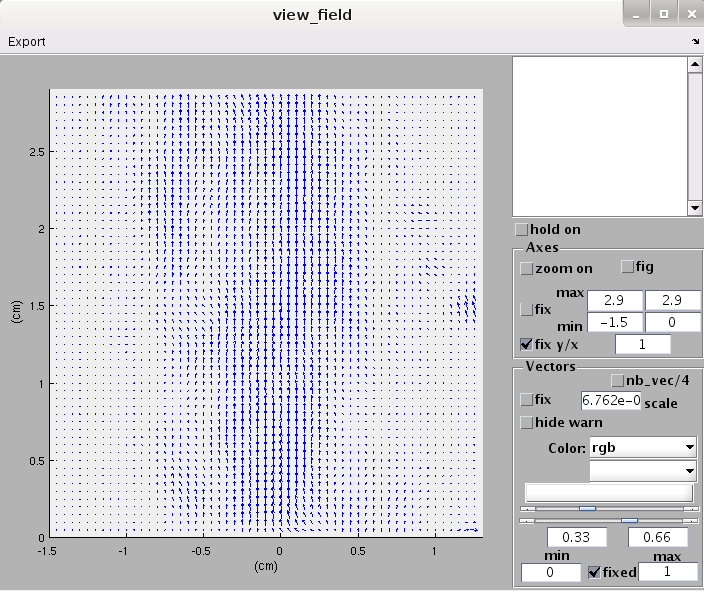
} { Vectors} To read the velocity field, open it with the GUI 'uvmat'. Velocity vectors are displayed in the central window, while the histograms of each component are in the lower left windows, see Fig. [uvmat_fig]. The arrow length is automatically set by default. It can be adjusted by the edit box [VecScale?] in the frame [Vectors'] on the right hand side.
The vector color indicates the quality of the image correlation maximum leading to each vector, blue is excellent, green average, red poor. The thresholds for such color display can be adjusted from 0 to 1 (perfect image correlation) in the frame [Vectors], using the boxes [ColCode1] and [ColCode2], or equivalently by the corresponding sliders [Slider1] and [Slider2] .
Vector color can also represent another quantity, as chosen in the menu [ColorScalar?] in the frame [Vectors]. For instance the vector length norm_vec can be used. Then a color continuous 64 color code is appropriate, as set in the menu [ColorCode?]. The color codes values between the valuies set by [MinVec?] and [MaxVec?].
The position (x,y) and velocity components (U,V) can be displayed in the upper right text display window by moving the mouse over it.
Derived fields
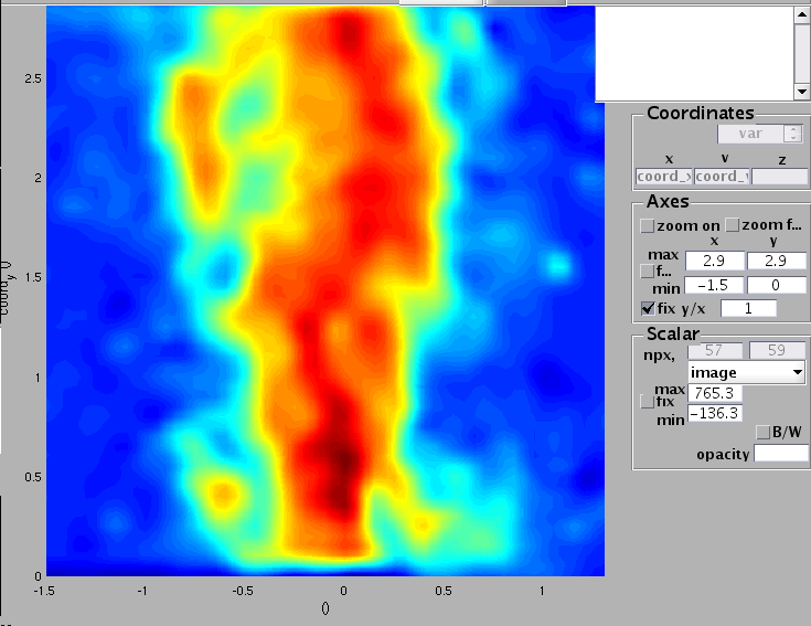
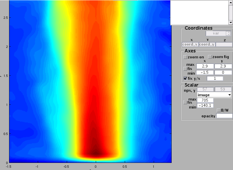
Other field representations are available, selected in the menu [Fields] at the top of the GUI. For instance the option 'u' provides a (false) color map of the x wise velocity component. A contour plot can be obtained instead of a color map by selecting the option 'contour' in the menu [ListContour?] in the frame [Scalar] . Then select the contour interval, for instance 0.5. The result is shown in the following figure. <doc145|center>
To get the vorticity field, 'vort' , and other spatial derivatives, you need to come back to the GUI CIV, select the check boxes [FIX1] and [PATCH1] , and press [RUN]. This will produce an interpolated velocity field and their spatial derivatives in the same netcdf file. After this operation vorticity can be visualized in the GUI uvmat, selecting the option [vort] in the popup menu [Fields]. The color code can be adjusted by the edit box [MinA] (saturated blue color below this value) and [MaxA] (saturated red color beyond this value).
Superposing image and vectors
It can be useful to visually superpose the images to the velocity field. This is done by selecting the option 'image' in the popup menu [Fields_1], located just under the popup menu [Fields] in the upper frame [Input]. To remove the image, select the blank option in [Fields_1] .
Similarly, the velocity vectors can be superposed to the vorticity field, selecting [vort] in [Fields_1] instead of [image .
Profiles
The velocity profile along a line can be obtained by creating a line with the upper menu bar [Projection object/line]. Then press the left hand side mouse button and draw the line, keeping the button pressed. Release the button to stop the drawing. The transverse and longitudinal velocity components along this line are then plotted in a new figure view_field.
Histograms
The global histograms of the displayed quantities (vector components or image brightness) are available in the lower left windows. Histograms limited to a sub-region can be extracted by the menu bar tool [Projection object], selecting either [rectangle], [ellipse] or [polygon] to define the sub-region. Then draw the contour with the mouse, like for line profiles.
Attachments (3)
- Tutorial7 - Civ on grid.png (29.9 KB) - added by 11 years ago.
- Tutorial7 - merge proj.png (61.4 KB) - added by 11 years ago.
- Tutoriel7 - Turbo stat.png (37.3 KB) - added by 11 years ago.
Download all attachments as: .zip