
TracNav
- Tutorial7: Correlation Image Velocimetry for a turbulent series
- Tutorial1: Image display
- Tutorial2: Projection objects
- Tutorial3: Geometric calibration
- Tutorial4: Processing image series
- Tutorial5: Correlation Image Velocimetry: a simple example
- Tutorial6: Correlation Image Velocimetry: optimisation of parameters
- Tutorial8: Correlation Image Velocimetry: advanced features
- Tutorial9: Image Correlation for measuring displacements
- Tutorial10: Image Correlation for steroscopic vision
- Tutorial11: Correlation Image Velocimetry with 3 components
- Tutorial12: Comparaison with a Numerical Solution
Tutorial 7 / Correlation Image Velocimetry for a turbulent series
This example applies Particle Image Velocimetry (PIV) to a turbulent jet, see TutorialParticleImageVelocimetry for a first introduction to PIV.
Visual check
Launch the GUI uvmat and open an image in 'UVMAT_DEMO03_PIVchallenge_2005C/images' , which represents a jet (images from PIV challenge, ref...). Images are organized in pairs, denoted with labels a, b with a short time interval Dt=0.01 ms, with interval 2 ms between two successive pairs. The timing and geometric calibration has been provided in the xml file 'images.xml', in the same way as discussed in the introductory example of tutorial 5.
Check the image pair between a and b, then between 1 and 2, dt is displayed while the time is displayed in the upper right edit box.
Civ
Open the GUI series/civ_input and import the processing parameters stored in 'UVMAT_DEMO03_PIVchallenge_2005C\Images.civ\0_XML\c001a.xml'
The seeding density is not excellent, so we keep the default correlation box [25 25]. The displacement in image pair is of the order of 1 to 2 pixels, so we use a small search box. The correlation box is slightly reduced for Civ2, [21 21] to improve the spatial resolution. A fairly low smoothing parameter is chosen for Patch to avoid smoothing of the inherently noisy turbulent flow. [RUN] the Civ1-Civ2 calculations using the default parameters.
Merge proj
To properly process data, a projection of the velocity fields on a grid is needed, preferentially in physical coordinates. Create this grid in the GUI uvmat by opening the velocity field determined earlier, then select [Projection object/plane] in the upper menu bar, and select [ProjMode]='interp_tps' in the GUI set_object. A grid mesh of 0.05 cm is proposed, corresponding to the vector density. Adjust the min and max in each direction for instance x=[-1.5 1.3] and y=[0 2.9]. Press [REFRESH] to see the result of the projection/interpolation on the grid. Press [SAVE] to backup the content of the GUI set_object as an xml file.

Now activate [Run/field series] in the upper menu bar of uvmat and select the [Action] function 'merge_proj'. Select the box [Projection Object] so that the plane in set_object is incorporated. If set_object has been closed, then open its backup as an xml file with the browser. Select the transform 'phys' in the menu [FieldTransform]. Select the indices i from first_i=1 to last_i=99. In the menu [FieldName] select simultaneously the options 'vec(U,V)', 'curl(U,V)', 'div(U,V)' (using the keyboard 'Ctrl' button). Note that the whole configuration of series can be retrieved by the menu bar command [Import Config], opening 'Images.ref.civ.mproj/0_XML/c_1-99.xml'. Press [RUN] to start the projection, preferably with [run mode]='background' to keep free the current Matlab session.
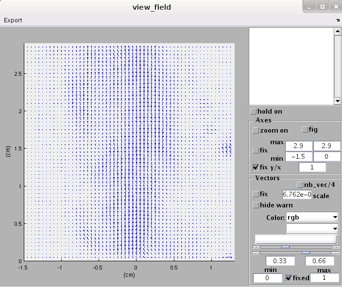
The projected fields are written as netcdf files in the folder 'images.civ.mproj'. Those can be opened by uvmat. The list of 'variables' appear in a GUI get_field. Selecting the variables 'U', 'V', 'curl'... in the table variables, we can see their dimensions in the right hand column. They are structured as two-component arrays (y,x) unlike the raw PIV results. Select the plot option 'scalar' or 'vector', and the quantity to plot in uvmat, as well as the variables used as coordinates, here 'coord_x' and 'coord_y'.

Turbulent statistics
From these files, basis turbulence statistics can be provided by the function turb_stat.m to be selected in the menu [Action] of series: select the option 'more...' which gives access to a browser from which this function, located in the folder 'UVMAT/series' can be selected. Then click on 'get_field' in [Fields] in series (right hand side), a new get_field GUI pops up. Select 'U' and 'V', click on [OK] and [RUN] the calculation in series.
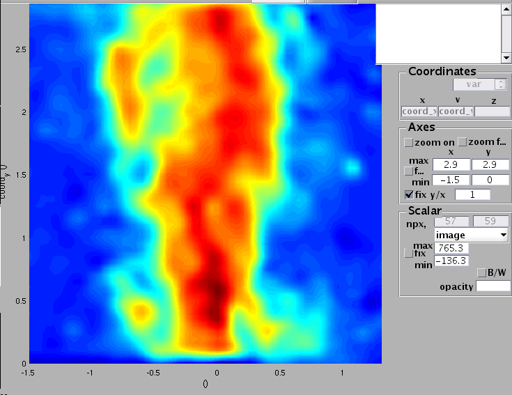
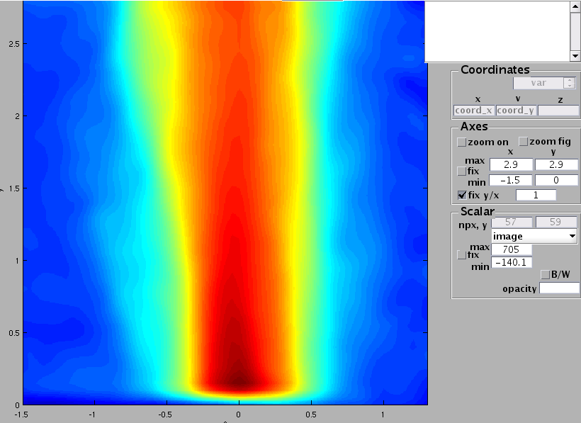
The result automaticaly shows up in uvmat and another get_field GUI appears, allowing to select the field coordinates: for instance the average of VMean gives the mean vertical velocity of the jet structure. The field uvMean clearly shows the structure of the Reynolds stress across the jet, if you create a [Projection object/line_x] on the result image you will clearly see that the curbe is positive on one side and negative on the other side, corresponding on the radial eddy diffusion of the jet.
The image below shows the VMean figure:

time series in a single netcdf file
For further data processing it can be convenient to merge all fields in a single netcdf file. This can be done by opening the previous results in series and applying the [Action] function 'time_series'. Select for instance the variables 'U' and 'V' as 'scalars'. No projection object is needed at this stage, so [Projection Object] must be unselected.
The result is obtained as a single netcdf file 'images.civ.mproj.tseries/c_1-99.nc'. Opening this file by uvmat, we observe that the arrays U and V are now with 3 components, (time, y, x). A plane of cut (x,y) is displayed in uvmat, whose z coordinate (here the time) can be moved by the [z slider] in the GUI set_object.
Attachments (3)
- Tutorial7 - Civ on grid.png (29.9 KB) - added by 11 years ago.
- Tutorial7 - merge proj.png (61.4 KB) - added by 11 years ago.
- Tutoriel7 - Turbo stat.png (37.3 KB) - added by 11 years ago.
Download all attachments as: .zip