
TracNav
- Tutorial12: Comparaison with a Numerical Solution
- Tutorial1: Image display
- Tutorial2: Projection objects
- Tutorial3: Geometric calibration
- Tutorial4: Processing image series
- Tutorial5: Correlation Image Velocimetry: a simple example
- Tutorial6: Correlation Image Velocimetry: optimisation of parameters
- Tutorial7: Correlation Image Velocimetry for a turbulent series
- Tutorial8: Correlation Image Velocimetry: advanced features
- Tutorial9: Image Correlation for measuring displacements
- Tutorial10: Image Correlation for steroscopic vision
- Tutorial11: Correlation Image Velocimetry with 3 components
Tutorial / Comparaison with a Numerical Solution
Introduction
Using synthetic images allows us to compare our PIV solution with the numerical one used to create the images. It is this way easy to determine the errors made during the PIC calculations.
The first part in this tutorial shows how to analyse perfect noise-free images and compare them with the synthetic solution. The next part will be focusing on creating noise in these same synthetic images and analysing them.
Synthetic Images
In the folder 'UVMAT_DEMO08_deformation', select one of the images from the 'a3b' series. It shows a diagonal uniform flow running from the bottom left corner to the top right one. [RUN] a PIV on the images series only using [CIV1], [FIX1] and [PATCH1] with the default parameters. Then [Open] one of the vector files (.civ) created. We need to substract the numerical solution to this image in order to keep only the errors between our calculation and the theorical one. Select the mall red square[SubField] under the [Input] table to open a second file in uvmat. Open the netcdf file of the synthetic solution 'a3b_sol_num.nc'. The GUI get_field pops up, select 'vectors' in the [FieldOptions] table and 'U' and 'V' in the right and left tables under [Ordinate]. The [Coordinates] should still remain as 'X' and 'Y'. Click on [OK]. An 'ERROR' window pops up, select [OK] and close the GUI set_object] which automatically popped up.
On the left hand side of uvmat select the [Tranform] function 'diff_vel'. If this one does not appear on the list, click on 'more...' and select 'diff_vel.m' from the folder 'UVMAT/transform_field'. A window will pop up asking about a scale factor for the second field, keep the default factor '1' and select [OK]. The difference between the two vectors should run automatically and the result appears in uvmat. Selecting [<-] and [+>] we can go through all the series observing the difference result on screen. A single file will be easier to observe the errors between the analytic and synthetic solutions. As we do not want to focus on the borders of the images we are going to create a [Projection object/rectangle] of [Max] (100, 100) with a center at x=128 and y=128. You can change these parameters once you drew the rectangle in set_object.
Then in order to obtain a single result file, go to series ([RUN/field series]). The two files should appear in the [Input Files] table. Select the [Action] function 'aver_stat'. A 'WARNING' window pops up ask you if you want to use a projection object, select [OK], the rectangle newly created should appear on the left hand corner under [Projection Object]. Another 'INPUT_TXT' window pops up to set the bin size for the histograms, enter '0.005' instead of 'auto' and select [OK]. Make sure that the i indices go from 1 to 41, that the [Field Transform] on the left hand side is 'diff_vel' and that the [VelType] in [Fields] (right hand side) is 'civ1' instead of '*'. It is possible to change the name of the file under [output SubDir], otherwise [RUN] the calculation.

Once it is done, the GUI get_field pops up again. Keep '1D plot' in the [FieldOptions] table and select 'UHisto' or 'Vhisto' in the [Ordinate] one. The [Coordinates] should change according to the input in the [Ordinate] ('U' if 'UHisto' is selected, same for 'V' and 'VHisto'). Select [OK].
A curve, close to a Gaussian, (gathering all the vectors from the difference between all the analytic and synthetic files of the series) appears in uvmat. See the .ref images to compare your result. On the right hand corner a table shows all the parameters of this curve. In the scroll bar [Field/get_field] it is possible to get back to the GUI get_field and change the [Ordinate]. You can also [Export] the curve [in new figure] or [on existing axis].
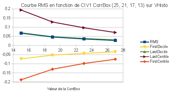
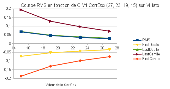
This is useful to determine and optimize some PIV parameters. The figure below shows the RMS, FirstCentile, FirstDecile, LastDecile and LastCentile of PIV calculations with different [CorrBoxSize].

Adding Noise
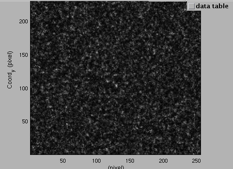
However as synthetic images do not exactly relate reality it is necessary to add noise to them in order to obtain a more realystic result. [Open] once again one of the 'a3b' images, then select the [Tranform] function 'ima_noise' (again if it does not appear on the list, click on 'more...' and select 'ima_noise.m' from the folder 'UVMAT/transform_field'). Some multiplicative noise is then added to the image.
As it is not possible to keep the [Transform] function 'ima_noise' while running a PIV we need to create another image serie with noise. To do that [RUN/field series] and select the [Action] function 'merge_proj'. Do not add any projection object, make sure that the [Field Transform] function is set as 'ima_noise' and that the calculation will run for all the images (from indice i=1 to i=41) and [RUN]. A new folder '.mproj' is then created with all the noisy images.

It is now possible to [Run] a [PIV] on this serie and by following all the steps from part1 (Synthetic Images) to obtain the difference between the analytical and noise solution and the synthetic one. The curve is not as smooth as in part1, you can indeed notice the effect of noise in a PIV calculation.
Adding an increment 'dt' in the PIV
In the folder 'UVMAT_DEMO08_deformation', select one of the images from the 'a2b' series. It shows a Lamb-Oseen vortex flow. In this part we are going to using the deformation CIV2 function and observe its effect on the calculations. To beginning with [RUN] a PIV on the images series only using [CIV2], [FIX2] and [PATCH2] with the default parameters. Then [Open] one of the vector files (.civ) created and substract it with the synthetic solution 'a2b_sol_num.nc' as in the first part of this tutorial.
Create a [Projection object/ellipse] of radius (50, 50) with a center at x=128 and y=128. You can change these parameters in set_object.
Finally [RUN/field series] with the aver_stat [Action] function and the [Projection Object] as before.
Now, [RUN] again the exact same PIV and select the deformation checkbox in [CIV2]. The calculation should take more time. Create the aver_stat field as well using the same projection object.
You now have the fields of the image series with and without deformation for dt = 1 (default parameter). Do the same calculations by selecting different values of [Di___:dt___] in [Pair Indices] on the top part of civ_series.
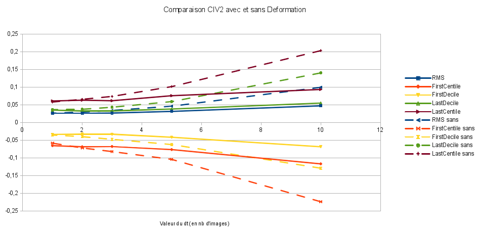
You will then be able to use the '.stat' fields to compare the effect of the deformation function in CIV2. The figure below shows the RMS, FirstCentile, FirstDecile, LastDecile and LastCentile of PIV calculations with different values of [Di___:dt___], with and without (=sans) deformation.

Attachments (5)
- Tutorial12-Aver_Stat.png (40.9 KB) - added by 11 years ago.
- Tutorial12-Noise.png (137.3 KB) - added by 11 years ago.
- Tutorial12-CorrBoxAnalysis.png (28.5 KB) - added by 11 years ago.
- Tutorial12-CorrBoxAnalysis2.png (28.6 KB) - added by 11 years ago.
- Tutorial12_deformation.png (52.5 KB) - added by 11 years ago.
Download all attachments as: .zip