Tutorial / Image display

Opening an image

Then type 'uvmat' in the Matlab command window, the GUI (Graphic User Interface) opens with the date of last modification. If the command '>>uvmat' is not recognized, check the Installation.

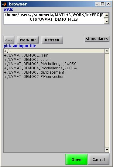
Activate the menu bar command [Open/Browse...] at the upper left which displays a file browser, as shown in figure.

Move through your computer folders (use '+/..' to move upward in the tree) to select the image file of the tutorial 'UVMAT_DEMO01_pair/images/frame_1.png'. The image should appear as in figure.

.

Open the folder UVMAT_DEMO01_pair containing the demo files, either form the downloaded archive (accessible on ​http://servforge.legi.grenoble-inp.fr/pub/soft-uvmat/), either online in the OpenDAP address http://servdap.legi.grenoble-inp.fr/opendap/meige/18UVMAT_DEMO_SOURCES/UVMA_DEMO001_pair (directly accessible in the menu [Open/Browse?...]). Then select the folder 'Images' and the image' frame_1.png'.

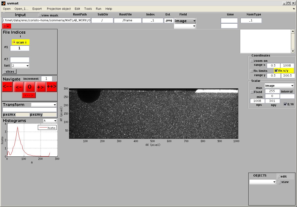
The file name is displayed in the upper frame [Input], split in path '.../UVMAT_DEMO01_pair' (in [RootPath]), subfolder '/images' (in [SubDir]), root file name '/frame' (in [RootFile]), index string '_1' (in [Index]) and file extension '.png' (in [Ext]). The file index is also displayed in the left frame [i1]. You can move to the next image 'frame_2' by pressing the red arrow [+>].

The box [NomType] indicates the convention for indexing, here using a separator '_'. It shows the first term in the series, which is '_1', while [FileIndex] is incremented when we move to frame_2 or beyond.

Brightness and contrast

The frame [Scalar] on the right hand side indicates the number of pixels (1008, 301) ([npx, y]) along the x and y directions, as well as the min and max brightness of the image (0 and 255). It is possible to change the brightness and contrast of the image display by setting values for these extrema. Pixels with brightness larger than the maximum will appear in white while pixels with brightness lower than the minimum will appear in black. The image histogram (number of pixels for each brigthness value A), is given in the lower left graph.

True color image

Let us choose now a color image as input, for instance UVMAT_DEMO02_color/images/frame1.jpg'. We notice in this example that the frame index '1' directly follows the [RootFile] 'frame' (without separator '_'), so [NomType] is '1'. By moving the mouse over the image, we notice that the luminosity A has three color components rgb (red, green, blue), shown in the upper right text window. Similarly the histogram has three curves.

Zooming

When zoom on is selected (tag=[CheckZoom]), zoom in by pressing the left side button of the mouse on the image and zoom out by pressing the right button. Use the key board directional arrows to adjust the field of view. It is also possible to manually write the coordinate limits by editing the boxes [MinX],[MaxX] and [MinY],[MaxY] in the frame [Axes]. To come back to the whole image, unselect the check box fix ([CheckFixLimits]).

A zoomed region can be also extracted as a separate figure by selecting zoom fig (tag [CheckZoomFig]) and drawing the contour with the mouse (keeping the left hand mouse button pressed). The zoomed region can be moved with the keyboard arrows.

Selecting the check box fix maintains the bounds fixed when different images of fields are opened (useful for comparisons), while the opposite option allows the bounds to adjust to the extremal coordinates of the field. Finally the x/y scaling can be set equal by selecting the box fix x/y (tag name [CheckFixAspectRatio]). Otherwise the image is deformed to fit in the plot window.

Edit boxes in the GUI can be also zoomed by right hand mouse button selection: a new window appears with the tag name and content. This is convenient when a text box content exceeds its frame limits (for instance RootPath).

Extracting data

The current mouse coordinates in the image, as well as the local image intensity ('A'), are displayed in the upper right text window. The local image matrix indices 'i' and 'j' are also displayed. By default the coordinates are expressed in pixel units, with origin (0,0) at the lower left of the image (the lower left pixel centre is at (0.5,0.5)). The x coordinate is equal to i-0.5 while the y coordinate is npy-(j-0.5), since the image index j runs from top to bottom unlike the coordinate y. In case of low screen resolution, it is possible to duplicate this display in a bigger window, by right mouse button selection inside the display area (after zoom has been desactivated).

When the mouse is over an edit box or press button, its tag is displayed with a short explanation (tooltip). The tag and box string can be also displayed by selection with the right hand mouse button.

The current image can be extracted for further processing with Matlab tools, for printing, saving, exporting etc. Use the menu bar command [Export/in new figure]. It can be also exported in the Matlab Command window as a Matlab variable (a structure), using the menu bar command [Export/as field in workspace]. The displayed field is represented by the sub-structure Data_uvmat.Field available in the workspace: the image matrix is Data_uvmat.Field.A while the X and Y coordinates of the first and last pixels are represented by Data_uvmat.Field.AX and .AY respectively.