
| Version 14 (modified by , 12 years ago) (diff) |
|---|
TracNav
- Tutorial3: Geometric calibration
- Tutorial1: Image display
- Tutorial2: Projection objects
- Tutorial4: Processing image series
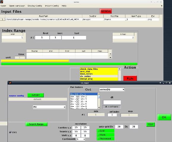
- Tutorial5: Correlation Image Velocimetry: a simple example
- Tutorial6: Correlation Image Velocimetry: optimisation of parameters
- Tutorial7: Correlation Image Velocimetry for a turbulent series
- Tutorial8: Correlation Image Velocimetry: advanced features
- Tutorial9: Image Correlation for measuring displacements
- Tutorial10: Image Correlation for steroscopic vision
- Tutorial11: Correlation Image Velocimetry with 3 components
- Tutorial12: Comparaison with a Numerical Solution
Tutorial / Geometric calibration
Simple scaling
Open again a test image in 'UVMAT_DEMO01_pair'.(accessible on http://servforge.legi.grenoble-inp.fr/pub/soft-uvmat/)
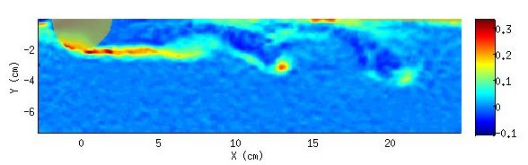
We shall use the diameter of the half cylinder visible on the upper let of the image to set the calibration. Its physical diameter is 2cm. The corresponding diameter in pixels can be obtained with the ruler displayed by the menu bar Tools/ruler of uvmat.
First zoom on the cylinder to optimize the precison. Select zoom on, press the left mouse button and adjust the field with the directional key board arrows. Then unselect zoom on to allow for other mouse actions (otherwise zoom has priority). It is also useful to increase the contrast at the cylinder edge by setting MaxA to 100 in the frame Scalar (right side of uvmat).
Then select the menu bar Tools/ruler, press the left hand mouse button on the cylinder edge, draw a diameter keeping the mouse pressed, release it on the opposite edge. The length in pixels, 140, is displayed, so the scaling factor is 140/2=70 pixels/cm.
Open the menu bar Tools/geometric calibration. A new GUI geometry_calib appears on the right side. Activate the upper menu bar Tools/Set scale on this GUI and introduce the value 70 in the edit box which pops up, and validate with OK. A set of calibration point coordinates appears in the table [ListCoord] of the GUI.
To see the calibration points on the image, first display the whole image by unselecting fix (tag [CheckFixLimits]) in the frame Coordinates of uvmat. Then press PLOT PTS in geometry_calib.
To perform the calibration, press APPLY, first with the default option 'rescale' in calib_type. The image is now displayed in phys coordinates. A xml file 'images.xml', containing the calibration parameters and reference point coordinates, has been created in the folder 'UVMAT_DEMO01_pair' (it should be identical with the file 'images.ref.xml' put for reference).
Note that the xml file name reproduces the name of the folder containing the images, so that images from different cameras should not be
Translating the coordinates
The origin of the phys coordinates is now arbitrary. It is more convenient to have it for instance at the centre of the cylinder, now at (x,y)=(1.69, 4.05).
To get the precise position of the cylindre, it is useful to introduce a projection circle, using in uvmat the menu bar command Projection object/ellipse. In set_object, select ProjMode='none', so that the line is just used as a marker, without projection operation. Set XMax=1, YMax=1, the radius of the circle, and the coordinates (1.69, 4.05) of the centre in the table Coord. Then press REFRESH. To optimise the visualisation, zoom in and increase the image contrast to MaxA=100.
To shift the coordinates, activate in geometry_calib the menu bar command Tools/Translate points, and fills (x=-1.69, y=-4.05) in the edit box which pops up. the phys coordinates of the calibration points are then shifted, and a new calibration put the cylindre centre at the origin (0,0).
put in the same folder.
Repeating the calibration
To repeat the calibration for several image series obtained with the same camera at the same position, different methods can be used.
-Copy the xml to the appropriate location, with the same name (but extension .xml) and path as the flle containing the image series. This is however not appropriate in general as the xml file contains other information, in particular about image timing.
-Open with uvmat one of the image of the series to calibrate, select Tools/geometric calibration, and in the GUI geometry_calib, the menu bar Import/All?, then press APPLY. For further repetitions, the GUI geometry_calib can be left opened while new image series are opened, and APPLY repeated each time without importing the calibration data again.
-In case of many image series, use RELICATE instead of APPLY in the GUI geometry_calib. Then select the 'campaign' to calibrate, i.e. the folder containing the series of experiments. Then in the new GUI browse_data, select the set of experiments and the corresponding set of data series to which the calibration must apply (this is used like Open campaign in uvmat).
Calibration with reference points
The more general method of calibration consists in using a set of reference points whose physical coordinates are known. Open with uvmat an image in 'UVMAT_DEMO06_PIVconvection/Dalsa1' (accessible on http://servforge.legi.grenoble-inp.fr/pub/soft-uvmat/)
Select in the menu bar Tools/geometric calibration. Mark the four box corners of the box with the mouse (left hand button). Their coordinates in pixels are displayed in the two last column of the table ListCoord in the GUI geometry_calib. To clear the table for corrections push the button CLEAR_PTS, or for a single line, use the key board backward arrow. To improve the position on the image, use the zoom and directional arrows. We find the coordinates of the four calibration points in pixels:
(X,Y)=(80.3, 81.6), (982.3, 86.1), (978.9, 937.4), (71.2, 929.5).
The corresponding physical coordinates are known to be
(x,y)=(0,0),(58.8,0),(58.8,55.1),(0,55.1), with an origin (0,0) taken at the lower left (and z=0).
Introduce those in the two first columns of the table [ListCoord]. This can be conveniently done by copy-paste Matlab vector x=[0 58.8 58.8 0] in the upper line of the x column, and y=[0 0 55.1 55.1] in the y column (use carriage return to validate the input).
To perform the calibration, press APPLY, first with the default option 'rescale' in calib_type. The image is now displayed in phys coordinates. We observe that the rectangular frame is slightly rotated. Furthermore the displayed precision, about 3 pixels, is not excellent.
To improve the precision we then apply the option 'linear' in calib_type, which seeks a general linear transform, including rotation. The precision is indeed improved to about 1 pixel. The previous xml file has been saved with a ~, ('Dalsa1.xml~') so it can be reverted in case of error.
Calibration with a target grid
Most precise and general calibration relies on the use of a target grid. As an example, open in uvmat the image ima_6 in 'UVMAT_DEMO07_GeometryCalibration/Dalsa1' (accessible on http://servforge.legi.grenoble-inp.fr/pub/soft-uvmat/). Open the menu bar Tools/geometric calibration and pick four corner points ABCD with the mouse define the periphery of the phys grid selected for calibration. The first point A will define the phys axis origin while AB defines the x axis and AD the y axis. AB and DC should be parallel on the phys grid (see fig). Then select Tools/Detect? grid on the upper menu bar of geometry_calib: you get a new GUI detect_grid in which you define (in phys units) the grid mesh and the positions of the first and last points on each axis. A z position can be defiend as well, do not fill it in this example. The option white markers is selected (by default) indicating that the grid is white (the opposite option would be needed for a grid made of black crosses on a white background). After validation by OK, the detected grid appears on uvmat (see fig).
If a point is not correct, select the option [CheckEnableMouse] in geometry_calib. Then you can adjust the point marker by selecting it with the (left button) mouse and moving it while keeping the mouse pressed (when adjustement is finished, nselected the option [CheckEnableMouse] to avoid spurious point creation with the mouse).
If the grid image is of poor quality, it is alternatively possble to mark all the points by the mouse, using the Tools/Create? grid instead of Tools/Detect? grid in geometry_calib (not convenient in general).
Once the grid has been marked, the calibration can be performed by the press button APPLY. We observe that the simple option 'rescale' is not appropriate in this case: a perspective effect is clearly visible, together with a non-linear deformation (grid lines are curved on the image). Therefore select the option '3D_quadr' which applies a 3D projection and quadratic correction. The grid image now appears of good quality in phys coordinates.
Merging the images of several cameras:
3D calibration :
The previous calibration corrects for 3D projection effects and gives some 3D indication. This is however made more precise by introducing different views of the same grid with different orientations, like shown in mages 1 to 5.
z position
Setting laser slices:
Attachments (10)
- Civ_1.JPG (51.4 KB) - added by 11 years ago.
- civ1_test.jpg (64.0 KB) - added by 11 years ago.
- Calib.JPG (40.5 KB) - added by 11 years ago.
- contours.JPG (29.6 KB) - added by 11 years ago.
- movie1-2.JPG (20.3 KB) - added by 11 years ago.
- vort_civ3-2.jpg (19.9 KB) - added by 11 years ago.
- vort_vel_zoom.jpg (97.5 KB) - added by 11 years ago.
- 3D_view.pdf (206.2 KB) - added by 11 years ago.
- Tutorial3 - Detect Grid (138.0 KB) - added by 11 years ago.
- 3D_view(1).pdf (239.6 KB) - added by 11 years ago.
Download all attachments as: .zip