Tutorial / Correlation Image Velocimetry: optimisation of parameters

To improve the results from the previous tutorial, open again in the GUI series, and enter the file frame_1.png in UVMAT_DEMO01_pair/images. Select the ACTION 'civ_series' which opens the new GUI civ_input. You may import existing processing  parameters by pushing the button ImportParam !ImportParam? at the top left of the GUI civ_input: open the parameter file images.civ/0_XML/frame_1.xml in the browser, or fill the GUI by hand as follows.

Time interval

The first parameter to adjust is the time interval between images, which should be sufficiently long to provide a displacement of a few pixels. The measurement precision is typically 0.2 pixel, so that a displacement of 4 pixels, as in the example, provides a relative precision of 5 %. A larger displacement would be preferable in terms of precision but may yield to poor image correlation and ’false vectors’. The choice of image pair is done in [!!ListPairCiv1].

Parameters for Civ1

Once the image pair has been chosen, the next parameter is  the size of the correlation box in both directions ([num_CorrBoxSize]_1] and _2), expressed in pixels. A smaller box of course improves the spatial resolution but it involves less statistics and false vectors may result from holes in the particle seeding. The particles are densely packed in this example, so we can significantly reduce the size from the default value [25,25] to [19,13] (in image pixels).  The use of a elongated box along x allows to optimize the resolution in the direction y, to deal with the transverse shear.

The next parameters are  ([num_!SearchBoxSize_1] and _2) and [num_SearchBoxShift_1], and _2, which determine the box in which the sub-image of the first frame is allowed to move to match the second frame. This can be adjusted from a prior estimate of the extrema of each velocity component (expressed in pixel displacement). Introduce  [min, max] =[ -2; 6] for ’u’ and [-3; 3] for ’v’, and press the button [Search Range]. The optimum search ranges and shifts (for the given correlation box) are now displayed: [33 25] and [2 0] respectively.

The PIV operation is conveniently visualised by pressing the button [!TestCiv1] in the GUI civ. Then the image appears in a new GUI view_field, in which the mouse motion displays the correlation function as a color map in a secondary window. The resulting vector is shown as a line pointing to the correlation maximum. The corresponding correlation and search boxes are shown in the image.

Unselect all operations except Civ1 and validate the parameters by pressing [OK]. Then run 'civ_series' in the GUI series and look at the result by pressing [STATUS], and open the .nc result file.

To observe the influence of the search box, come back to the GUI civ_input, set [CorrBoxSize]=[19 13] and [SearchBoxSize]=[27 25] with [Shift]=0, and visualise the result with uvmat. Many black vectors (F=-2) are obtained, showing that the search domain is too small, so that the correlation maximum is constrained by the limited search interval. Using [!TestCiv1] , it can be seen that the correlation maximum is indeed at the edge of the Search box in the main flow with u$\simeq$4 (while a gap of 2 pixels is required to properly determine the maximum without edge effect).

of research of the expressed in pixels. For each velocity vector, the correlation box is moved within the search box to optimise the image correlation between the two sub-images inside the correlation box. To allow for a displacement of d pixels, the search box size must exceed the correlation box by at least d+2 on both sides, so 2d+4. A systematic shift  can be also introduced to minimise the search area in the presence of a mean flow.

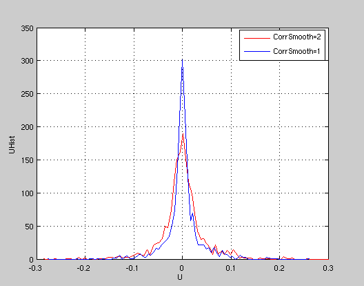
The parameter [num_CorrSmooth] is used to fit the correlation data with a Gaussian function to obtain the maximum with sub-pixel precision. We generally keep the default value 1, while the value 2 should be more appropriate for larger particles (with wider correlation maximum).

The parameters [num_Dx] and [num_Dy] define the mesh of the measurement grid, in pixels. Reduce them to get more vectors, but keep in mind that the spatial resolution is anyway limited by the size of the correlation box, so that velocity vectors become redondant when the sub-images highly overlap those of the neighboring vector. Then the choice Dx=Dy=10, about half the correlation box, provides a good optimum.

Finally select the Mask option like in the previous tutorial.

FIX1:

Select the ’FIX1’ operation, which eliminates some false vectors using several criteria. Use the default parameters.

PATCH1:

Select the ’PATCH1’ operation, to interpolate the vectors on a regular grid and calculate spatial derivatives. Choose the default value 10 for the smoothing parameter [FieldSmooth]. You can later try different values, the smoothing effect increasing with [FieldSmooth]. Keep the default values for the other parameters.'

CIV2:

Select the ’CIV2’ operation to improve the correlation results, using the information on local image deformation, provided by the previous knowledge on velocity spatial derivatives (calculated in patch1). Use a finer grid dx= dy=5 than for civ1. The spatial resolution can be slightly improved by decreasing the correlation box, using for instance Bx,By=(15,11). The shift of the search range is here given at each point by the prior estimate from Civ1, so that the search range can be optimized: choose [21,17] which provides a margin of 3 pixels on each side of the correlation box. Note that ’civ2’ corresponds to a new measurement from the images, the previous civ1 and patch1 operations being used only as an initial guess for the search of optimal correlations.

FIX2 and PATCH2

Then select ’FIX2’ and ’PATCH2’ with the default parameters.

Further Civ iterations

The parameters of a CIV computation are stored in a xml file with extension ..CivDoc.xml created in the directory containing the velocity files. These parameters can retrieved, opening this xml file with the browser of the GUI civ. Then the image file itself needs to be opened (the select again the check boxes for the operations beyond civ1 hidden by default).

The result can be improved again by performing a third civ iteration, civ3. For that purpose, select only the ’civ2’, ’fix2’ and ’patch2’ operations with the same parameters as previously. The previous result is now considered as ’civ1’, so set CIV as the subdirectory in the edit window [SubDirCiv1]. Select a new subdirectory name, for instance ’CIV3’ in the edit window [SubDirCiv2]. Further iterations could be similarly performed, but the improvement becomes negligible.

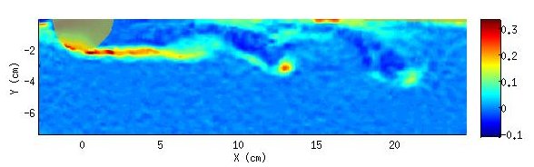
The following figure shows the final vorticity field, in which the vorticity roll up in the wake of the sphere is clearly visible. A zoom near a vortex shows the vorticity superposed with velocity vectors.